Introduction
In this exercise, we will conduct a nonlinear static analysis to explore the phenomenon of stress stiffening. The subject model is a flat walled tank that is 48 inches x 48 inches x 96 inches tall. The walls of the tank are flat and are subject to pressure loading which may lead to large deformation effects.
We will run this analysis as both a linear static and a nonlinear analysis and compare the results.

1. Open the Model and Start the Autodesk Nastran In-CAD Environment
Start Autodesk Inventor, and open Flat Walled Tank.ipt from the Section 15 - Flat Walled Tank sub-folder of your training exercises folder.You should see this:
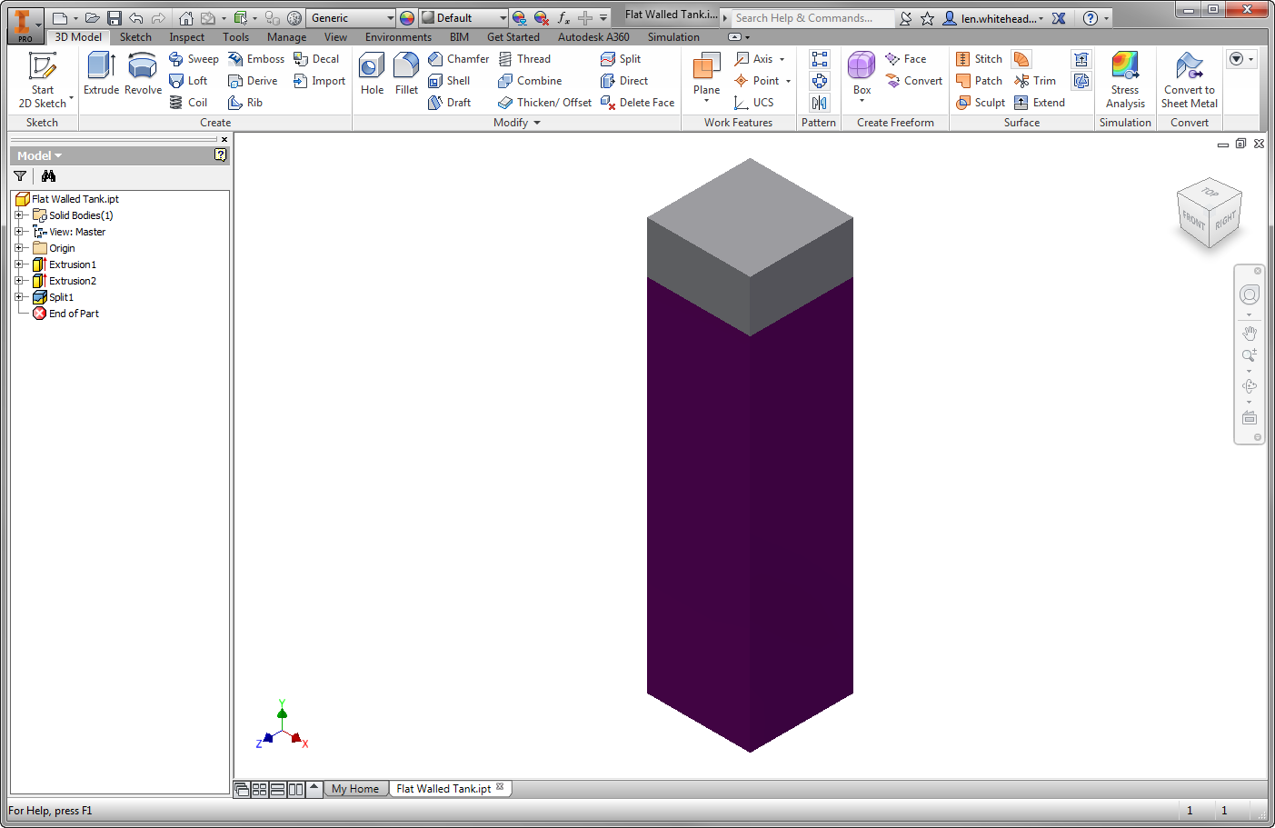
Note that this model is a quarter of the actual tank. This reduces the model to a 1/4 symmetry. Also note the feature called Split1. This is how we will control the liquid fill height of the tank. We will assume a fill height of 84 inches. Note that the "wetted" faces that experience the pressure load are colored purple.
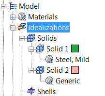
From the Environments ribbon tab, click Autodesk Nastran In-CAD. In the Model tree, expand Idealizations. If any Idealizations are already defined, like Solids 1 and 2 below, right-click , to ensure that no unwanted materials can participate in the analysis.
2. Define the Physical Property
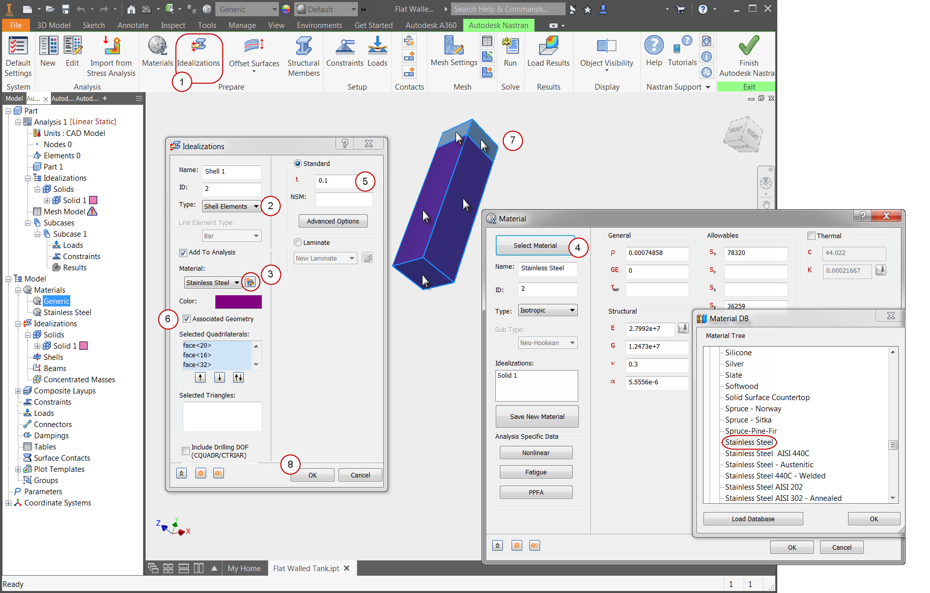
- Click Idealizations from the ribbon.
- On the Idealizations dialog, set the Type to Shell Elements.
- Click the New Material icon.
- On the Material dialog, click Select Material. Expand the Autodesk Material Library, and select Stainless Steel. Click OK. Click OK on the Material dialog.
- On the Idealizations dialog, set the thickness, t, to 0.1.
- Check the Associated Geometry box.
- Select the five surfaces on the tank as shown.
- Click OK.
3. Mesh the Tank
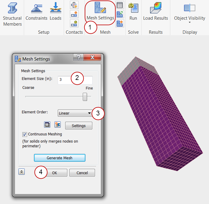
- Click Mesh Settings from the Mesh panel of the ribbon.
- Enter 3 as the Element Size.
- Change the Element Order to Linear.
- Click OK to generate the mesh.
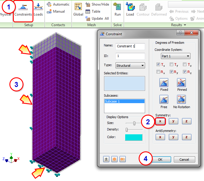
4. Constrain the Tank Edges in the YZ Plane
In this step, we will assign X symmetry to the symmetry edges in the YZ plane.
- Click Constraints from the ribbon.
- Click X Symmetry.
- Select the three edges shown in the image. Note the orientation of the model and the coordinate system.
- Click OK.
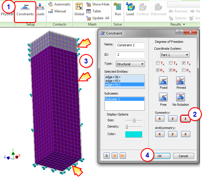
5. Constrain the Tank Edges
In this step, we will assign Z symmetry to the symmetry edges in the XY plane.
- Click Constraints from the ribbon.
- Click Z Symmetry.
- Select the three edges shown in the image. Note the orientation of the model and the coordinate system.
- Click OK.
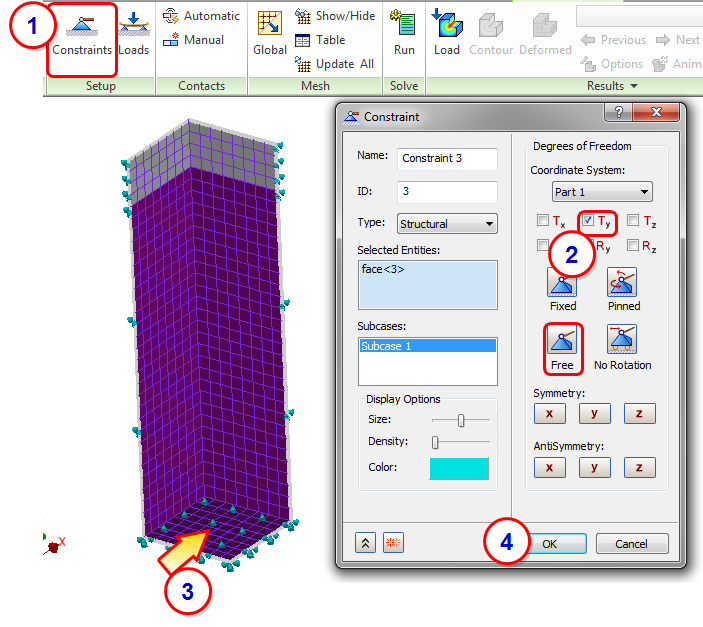
6. Constrain the Bottom of the Tank
Next we add a vertical constraint to the bottom surface to ensure the bottom surface stays on the ground. This and the two symmetry conditions allow the tank to expand naturally.
- Click Constraints from the ribbon.
- Click Free, and then Ty.
- Select the bottom surface of the tank.
- Click OK.
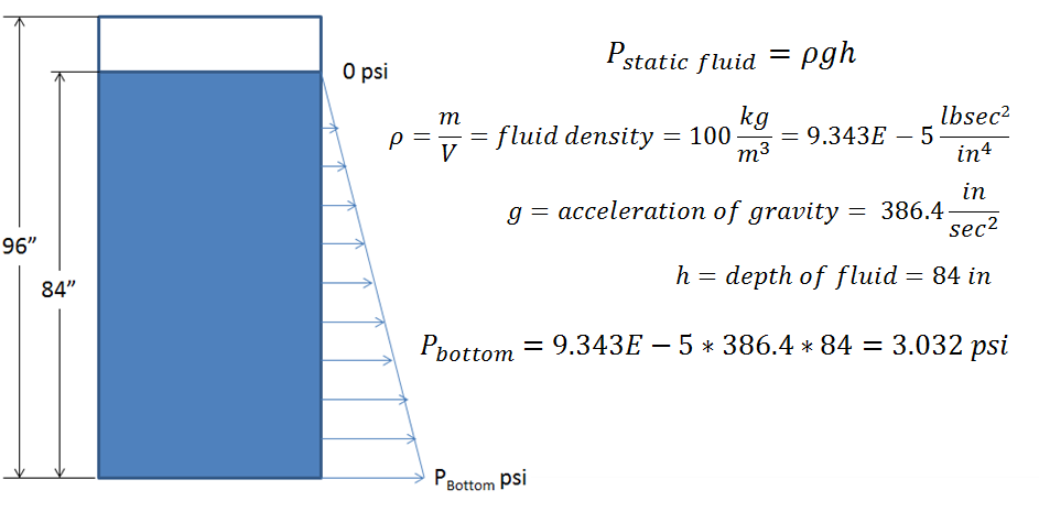
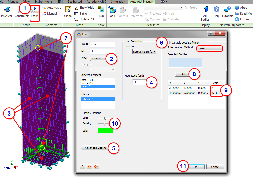
7. Assign the Pressure Load
By performing a simple hydrostatic analysis of the tank, we determine that the pressure at the bottom of the tank with an 84 inch column of water is 3.032 psi:
- Click Loads from the Setup panel of the ribbon.
- Select Pressure as the Type.
- Select the three wetted surfaces of the tank.
- Enter a Magnitude of -1.
- Click Advanced Options to expand the dialog so the Variable Load Definition is visible.
- Check Variable Load Definition, and ensure that the Interpolation Method is set to Linear.
- Select the two vertices shown, first the top one, then the bottom one.
- Click Add.
- In the Scalar column of the table, double-click in the top cell and enter 0 in row 1, and 3.032 in row 2.
- To see the varying load more clearly, in the Display Options area, move the Density slider.
- Click OK.
8. Run a Linear Static and Review the Results
- Click Run from the ribbon.
- From the Results branch of the Analysis tree, right-click on Displacement, and click Display.
- Right-click on von Mises, and click Display.
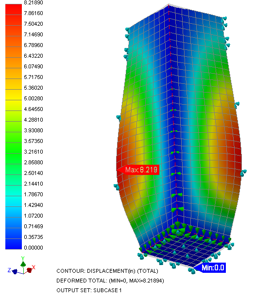
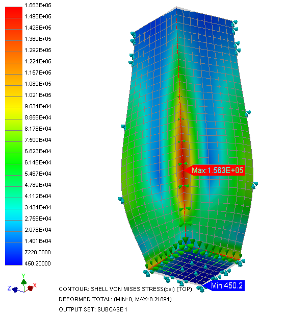
Both the displacement and the von Mises stress results plots show that there are problems with the tank.
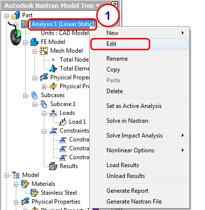
9. Change the Analysis Type to Nonlinear Static and Rerun
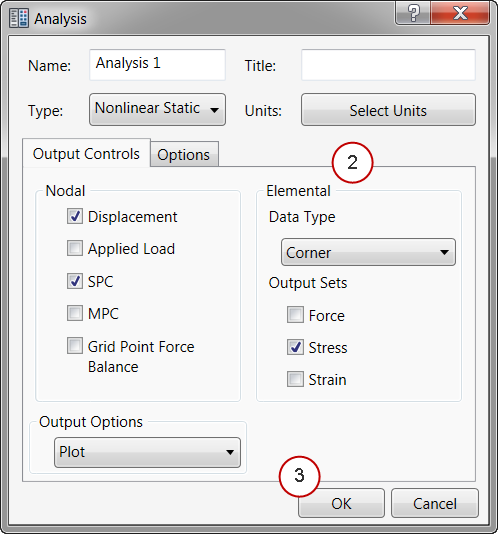
- Right-click on Analysis 1 in the Analysis tree, and click Edit.
- Change the Type to Nonlinear Static.
- Click OK.
- Click Run from the ribbon.
10. Review Nonlinear Results
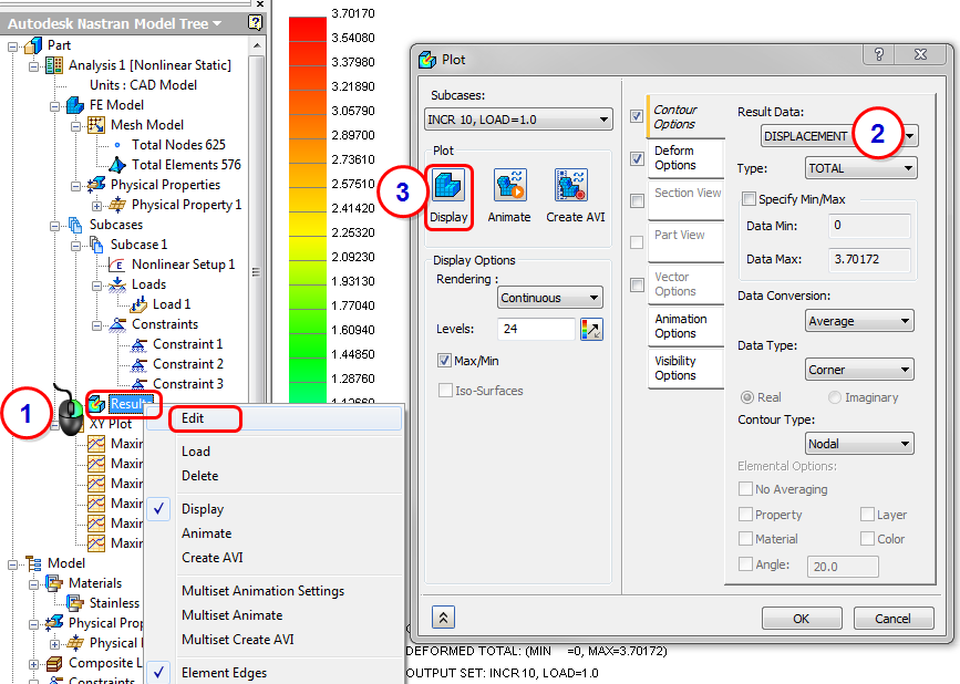
- Right-click on Results in the Analysis tree, and click Edit.
- Select Displacement.
- Click Display.
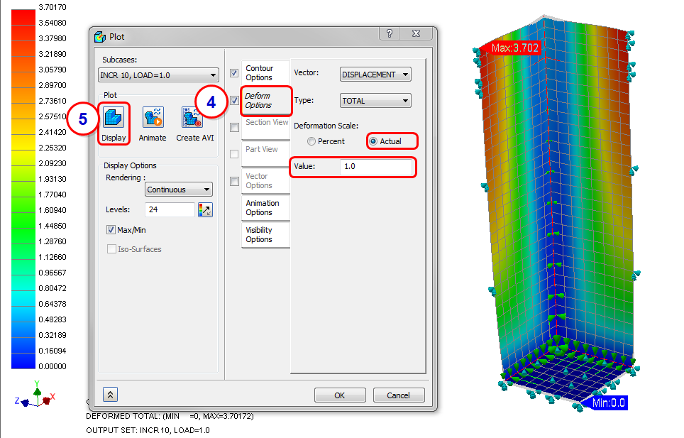
- Click the Deform Options tab. Select Actual, and specify a Value of 1.0.
- Click Display.
- Click the Contour Options tab. Change Result Data to Stress, and change Type to SHELL MAX VON MISES STRESS. (If the results do not update, click Display.)
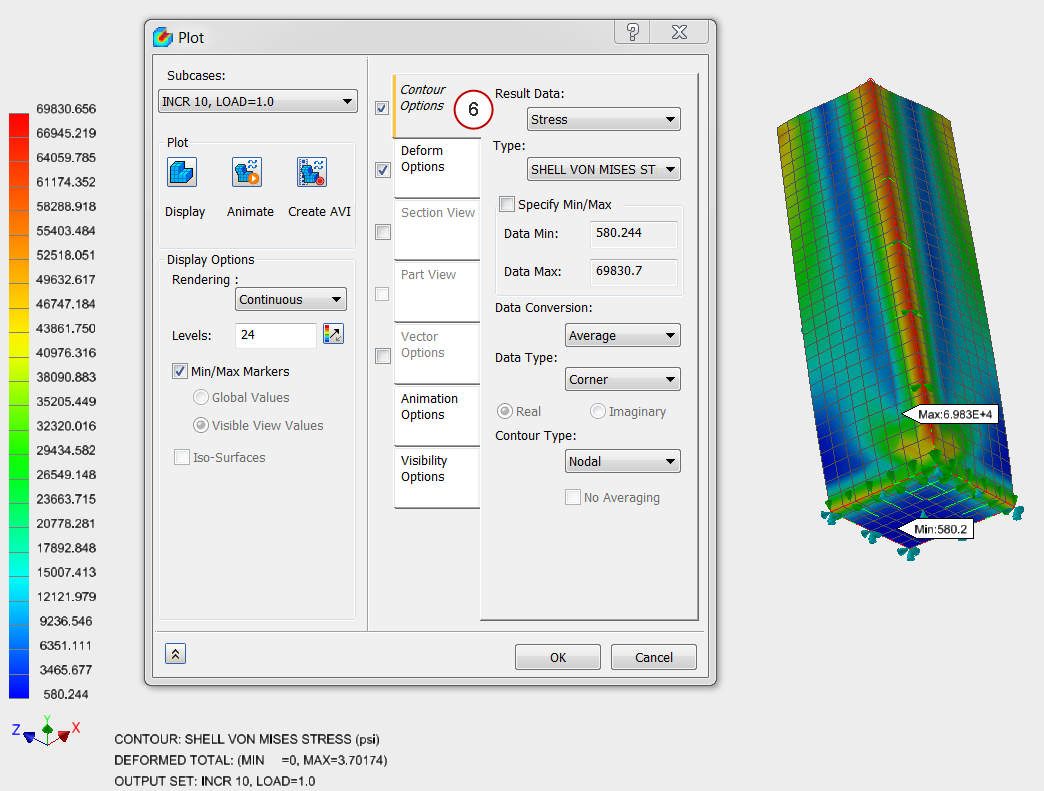
The results look significantly different from the linear static results!
Summary
In this exercise, we compared linear and nonlinear results for a large displacement model to demonstrate how we can obtain better accuracy by switching to the Nonlinear Static analysis type. Additionally, we used symmetry constraints on a shell model, and defined shell properties on a solid face. To simulate the variation of hydrostatic pressure on depth, we applied a varying load to the vertical wetted surfaces of the tank.
|
Previous Topic: Nonlinear Static Analysis |
Next Topic: Nonlinear Transient Analysis |