Element types used in structural analysis (Concept)

For Midplane and Dual Domain analysis technologies, structural analyses offer both shell and beam elements.

Shell Elements

Shell elements take the form of planar, straight-edged triangles. When modeling curved shells, they provide a "faceted" approximation to the true geometry. Currently, the thickness of each element is assumed to be constant, although the thickness of adjoining elements may be different.

In all cases, six displacement degrees of freedom are used at each node. These include, three translations parallel to the global axes and three rotations about these axes. For smooth shells it is possible to use only five degrees of freedom, that is three translations and the two local rotations of the mid-surface normal. However, the use of six degrees of freedom in all cases has distinct advantages.

It allows non-smooth structures such as boxes, trays and stiffened shells to be analyzed without applying any special constraint conditions to the junctions between intersecting surfaces.
Beam elements (which in three-dimensional space must have six degrees of freedom) can be attached directly to the nodes of the underlying plate or shell mesh without applying constraints or transformations.
In a large deflection (geometrically non-linear) analysis, the use of three rotational degrees of freedom allows an elegant and geometrically exact model for finite rigid body motion to be introduced [1-3].

It is worth noting that many of the deficiencies of existing geometrical non-linear models of thin-walled structures can be traced to approximations made with respect to the rotational parameters. The parameters adopted here are "natural" in the sense that they are directly related to spectral analysis of the associated rotation tensor. To obtain linearized forms, use is made of the classical analysis of rigid body kinematics by Euler and Rodriques [1,3,4].

The element formulations account for membrane, flexural and transverse shear deformations. The latter is based on the Reissner-Mindlin theory [5,6]. In this theory the classical Kirchhoff assumptions for thin plates and shells are relaxed by lowering the continuity requirements from C₁ to C₀ , including transverse shear. This allows both "thin" and "moderately thick" plates and shells to be modeled. In practice, the performance of such elements is known to deteriorate rapidly as the plate or shell becomes thin. This phenomenon is called shear locking and is caused by the inability of the element to approach the limiting condition of zero transverse shear strain at the appropriate quadratic rate. Shear locking is alleviated by the use of reduced integration, but contrary to early expectations [7], it is by no means eliminated.

More recently, variants of the energy balancing techniques introduced by Fried [8] and McNeal [9] have produced excellent results over a wide range of structural aspect ratios (ratio of a characteristic dimension measured around the mid-surface of the shell structure to the average wall thickness). The form used for the present triangular elements is due to Tessler and Hughes [10], and allows accurate results to be obtained over the approximate aspect ratio range:

Apart from eliminating locking, the method reduces sensitivity of thin shells to element distortion, and improves the conditioning of the stiffness matrix and the quality of stress prediction.

Note: The analogous problem of membrane locking only occurs in thin curved elements and therefore need not be considered here.

Currently, only linear elastic materials can be modeled. These maybe either isotropic or orthotropic. In the latter case, the principal planes of the material are orthogonal, with one plane lying in the mid-surface of the shell and the other two planes intersecting this surface along two perpendicular lines referred to as the directions of orthotropy. The directions of orthotropy are determined by processing and are prescribed for each element from the Fill+Pack analysis. The material properties in each direction are specified by the user when preparing the analysis inputs file for the Warp or Stress analysis.

Geometric non-linearity is based on a convected Lagrangian approach in which the displacement field is referred to a set of local convected coordinates that co-rotate with the cross-sections of the shell at each point. For consistency, the usual inextensibility condition is here applied to fibers that are collinear with the cross-sectional director at any point.

The co-rotational method derives from the polar decomposition theorem of continuum mechanics which asserts that any general spatial motion can always be decomposed into a pure stretch (deformation) followed by a rigid body motion. Adopting suitable finite rotation measures (see above) and explicitly discarding the rigid body component of the overall motion, a consistent method of evaluating the internal deformations and associated stresses within an element is achieved. In practice, this means that no limitations need to be placed of the magnitude of the rigid-body motion, and that the precision with which the internal deformations and stresses are determined will remain constant throughout the analysis.

The formulation is closely related to the finite deflection theories of Reissner [11,12], Simmonds and Danielson [13], Danielson and Hodges [14], and the finite element implementation of these theories by Bates [1] and Simo and Vu-Quoc [15].

Element LMT3

Element LMT3 is used in Midplane analysis technology. LMT3 is a three-noded triangular element with 18 degrees of freedom (six at each node). The element is constructed by superimposing the local membrane formulation due to Bergan and Nygard [16] and Bergan and Felippa [17] with the bending formulation due to Tessler and Hughes [10] and transforming the combined equations to the global coordinate system. The resulting element can model bi-linear variations of membrane and transverse shear strains, but the flexural strains (curvatures) are constant.

The "free formulation" of Bergan and Nygard is based on assumed displacement fields, but goes beyond the strict potential-energy formulation in allowing "nonconforming" shape functions to be used. To ensure convergence, patch test requirements are enforced a-priori. The displacement shape functions are separated into basic and higher-order modes, the former being associated with rigid body and constant strain states and the latter with coordinate invariant in-plane bending modes.

This leads in turn to a basic and higher-order stiffness denoted by

and

respectively. The combined membrane stiffness then takes the form:

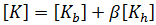
where is a free parameter that acts as a scaling factor on the higher-order stiffness. In line with detailed test results, = 1.5 has been adopted as the best choice.

The rotation about the local mid-surface normal (often referred to as the drilling freedom) is linked to the average in-plane rotation of the mid-surface by the penalty constraint technique. Thus,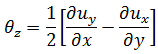

The drilling freedom is a fully integrated active component in the formulation. The strength of the link between and the in-plane gradients remains even in the case of exactly co-planar elements, so that singularity problems no longer occur. Great attention must be paid to the use of as a boundary condition component.

The basis of the bending formulation of the element is an explicit degree of freedom technique achieved via continuous transverse shear edge constraints [10]. This leads to a constrained (coupled) total displacement field with bi-quadratic variation in the lateral displacementu_z and bi-linear variations in the normal rotations and . When combined with the transverse shear correction factor technique [10], the element exhibits a much improved flexural response (compared to the standard constant curvature formulation) across a wide range of aspect ratios.

Element Definition

The geometry, node numbering and local/global degrees of freedom for the element are shown in the LMT3 Shell Element. Note that nodes i, j, k refer to entries in the nodal connectivity table given in the analysis output file. For example, if the connectivity for an element is 11, 101, 85 then i = 11, j = 101, k =85, and the local X-axis runs from node 11 to node 101.

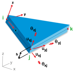
The LMT3 Shell Element

Element Loading

Two types of element loading are available: pressure loading and initial strains due to orthotropic shrinkage.

Pressure loads are assumed to act on and be normal to the element mid-surface. The pressure is assumed to have a constant value over any given element, although pressure values used in adjacent elements may be different.

Integration Rules

Integration over the mid-surface is carried out using three-point numerical quadrature. Since the material is linear elastic and the element is flat, both the strains and the stresses vary linearly through the shell walls. Consequently, explicit pre-integration in the thickness direction is used rather than the more expensive numerical integration.

The integration station locations and weights are shown in Integration station locations for LMT3 Element and Integration location weights for LMT3 Element.

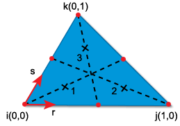
Integration station locations for LMT3 Element

Integration location weights for LMT3 Element
Element	Integration Station	r-coordinate	s-coordinate
LMT3	1 2 3	1/6 2/3 1/6	1/6 1/6 2/3

Results Output

Membrane forces 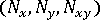, bending moments 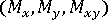and transverse shear forces are calculated at the integration stations and are illustrated in Results from Analysis for the LMT3 Element.

These results are reproduced in the analysis output file.

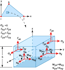
Results from Analysis for the LMT3 Element

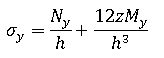
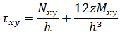
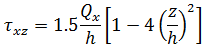
Assuming plane stress conditions, the stresses at any level z are given by: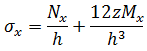

Note that the forces and moments are those acting on a unit width of the plate or shell and so the membrane and shear forces have dimensions force/length, whereas the moments have dimensions (force).

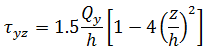
Element LBT3

Element LBT3 is used in Dual Domain analysis technology. LBT3 is a three-noded triangular element with 18 degrees of freedom (six at each node). The element is constructed by superimposing the local membrane formulation due to Bergan and Nygard and Bergan and Felippa with the bending formulation due to Batoz and transforming the combined equations to the global coordinate system. The resulting element can model bi-linear variations of membrane, flexural strains and transverse shear strains.

This leads in turn to a basic and higher-order stiffness denoted by

and

respectively. The combined membrane stiffness then takes the form:

where is a free parameter that acts as a scaling factor on the higher-order stiffness. In line with detailed test results, = 1.5 has been adopted as the best choice.

The rotation about the mid-surface normal (drilling freedom) takes the same continuum mechanics definition as that used for LMT3, that is,

The bending formulation of the element is based on the generalization of discrete Kirchhoff techniques to include the transverse shear effects. The element is free of locking, and valid for the analysis of thick or thin parts. It coincides with the well-known DKT (discrete Kirchhoff triangle) element if the transverse shear effects are not significant.

Numerical tests indicate the LBT3 performs very well. Generally LBT3 is slightly better than LMT3. In addition, both single-layer and multi-layer formulations are available in LBT3, but LMT3 is currently only valid for single-layer analysis.

The multi-layer LBT3 is recommended to be used to conduct Stress and Warp analyses of fiber-filled plastics. With the fiber orientation considered layer by layer, the physical model is more realistic and the result is expected to be more accurate.

Element Definition

The geometry, node numbering and local/global degrees of freedom for the element are shown in the LBT3 Shell Element. Note that nodes i, j, k refer to entries in the nodal connectivity table given in the analysis output file. For example, if the connectivity for an element is 11, 101, 85 then i = 11, j = 101, k =85, and the local X-axis runs from node 11 to node 101.

The LBT3 Shell Element

Element Loading

Two types of element loading are available: pressure loading and initial strains due to orthotropic shrinkage.

Integration Rules

The integration station locations and weights are shown in Integration station locations for LBT3 Element and Integration location weights for LBT3 Element.

Integration station locations for LBT3 Element

Integration location weights for LBT3 Element
Element	Integration Station	r-coordinate	s-coordinate
LBT3	1 2 3	1/6 2/3 1/6	1/6 1/6 2/3

Results Output

Membrane forces , bending moments and transverse shear forces are calculated at the integration stations and are illustrated in Results from Analysis for the LBT3 Element.

These results are reproduced in the analysis output file.

Results from Analysis for the LBT3 Element

Assuming plane stress conditions, the stresses at any level z are given by:

Note that the forces and moments are those acting on a unit width of the plate or shell and so the membrane and shear forces have dimensions force/length, whereas the moments have dimensions (force).

Beam Elements

The beam element BEAM2, which is a two-noded beam, is currently available in both Midplane and Dual Domain analysis technologies.

The longitudinal axis of the elements is straight, so that when modeling curved beams, they provide a "faceted" approximation to the true geometry. Currently, the beam is assumed to have a circular cross-section of constant radius. However, the cross-sectional radius of adjacent elements may be different.

Six degrees of freedom are used at each node, namely, three translations parallel to the global axes and three rotations about these axes. In the context of finite rotations, the rotational degrees of freedom have exactly the same definition as that discussed for shells. The physical connection of beam and shell elements at one or more nodes is straightforward. Note that if every beam node is attached to a shell node, then the total number of equations that are needed to model the combined structure is the same as the number required to model the shell structure on its own. Thus, the computational overhead involved in adding beam elements is generally quite small.

The element formulations account for axial, bending, torsional and transverse shear deformations. The basic assumptions are that the beam cross-section remains plane and undistorted but, in the presence of transverse shear, it will not remain normal to the longitudinal axis. The resulting model can be thought of as deriving from a classical Euler-Bernoulli beam in two stages. Firstly, the average effects of transverse shear are accounted for by adding a Reissner-Mindlin type shear model. This leads to what is generally referred as a Timoshenko beam. In the second stage, the torsional behavior is modeled using the theory due to St.Venant.

Where a runner, rib or stand-alone beam structure is modeled with beam elements, then the aspect ratio (ratio of total length measured along the axis of the beam to the average cross-sectional diameter) should lie in the approximate range:

The very high upper limit is made possible by using the penalty relaxation technique. Although the beam elements do not suffer from shear or membrane locking, this technique prevents the element stiffness matrix from becoming ill-conditioned at high aspect ratios.

Currently, only isotropic linear elastic materials can be modeled for beam elements. Note that it is not possible to account for general orthotropic material behavior without conflicting with the basic assumptions mentioned above.

The co-rotational method derives from the polar decomposition theorem of continuum mechanics which asserts that any general spatial motion can always be decomposed into a pure stretch (deformation) followed by a rigid body motion. Adopting suitable finite rotation measures and explicitly discarding the rigid body component of the overall motion, a consistent method of evaluating the internal deformations and associated stresses within an element is achieved. This means that no limitations need to be placed of the magnitude of the rigid-body motion and that the precision with which the internal deformations and stresses are determined will remain constant throughout the analysis.

The formulation is closely related to the finite deflection theories of Reissner [11], Danielson and Hodges [14], Hodges and Simo. The finite-element implementation of these theories by Bates [1] and Simo and Vu-Quoc [15] is also relevant.

Element BEAM2

This is a 2-noded beam with 6 degrees of freedom at each node. The beam axis is assumed to be straight and the cross-section to be circular and solid. The element can be used in stand-alone form or, alternatively, it may be connected to one edge of the triangular shell elements LMT3.

The formulation is based on linear isoparametric shape functions. To avoid shear locking, reduced integration is used to find the stiffness and internal forces, which in this case means using 1-point Gauss quadrature. The resulting model exhibits constant axial, bending, torsional and shear strain fields.

In its unmodified form, the predicted element response depends on the bending mode to which the element is subjected.

For pure bending, exact nodal displacements and stress resultants are obtained at the control integration point.

However, the over-stiffness in the latter case are completely eliminated by applying the penalty relaxation method [19]. Exact displacements and central stress resultants are also predicted for constant stretching and twisting.

Element Definition:

The geometry, node numbering and local/global degrees of freedom for the element are shown in the BEAM2 Beam Element. Note that nodes i, j refer to entries in the nodal connectivity table that is given in the analysis output file. For example, if the connectivity for an element is 55, 77 then i = 55, j = 77, and the local X-axis runs from node 55 to node 77.

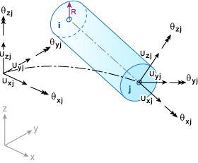
The BEAM2 Beam Element

Element Loading: The only type of element loading currently available is the specification of axial and curvature strains due to shrinkage. (Note, however, that concentrated external loads, that is forces and moments, can be applied directly to the nodes of the finite element mesh.)

Integration Rules

Internal forces (stress resultants) are calculated at the central integration point shown in Integration Station for BEAM2 Element and reproduced in the analysis output file.

For a linear elastic material, both the strains and stresses vary linearly over the cross-section of the beam. Consequently, explicit pre-integration over the cross-section is used instead of the more expensive numerical integration.

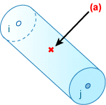
Integration Station for BEAM2 Element

(a) integration point.

Results Output

The following stress resultants are calculated at the integration station and reproduced in the analysis output file.

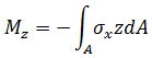
Moments: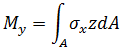

Torsion:

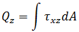
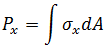
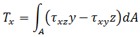Forces:

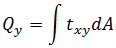
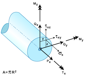
Results From Analysis for the BEAM2 Element

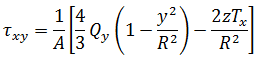
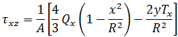
The stresses at any point (y,z) are then given by: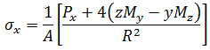

References

Argyris, J.H., "An excursion into large rotations", Comp. Meth. Appl. Mech. Engrg., Vol. 32, 1982, pp. 85-155.
Rankin, C.C. and Brogan, F.A., "An element independent corotational procedure for the treatment of large rotations", in: Collapse Analysis of Structures (L.H. Sobel and K. Thomas eds.), ASME, New York, 1984, pp. 85-100.
Bates, D.N., The mechanics of thin walled structures with special reference to finite rotations, Ph.D. Thesis, University of London, 1987.
Hodges, D.H., "Finite rotation and non-linear beam kinematics", Vertica, Vol. 11, No. 1/2, 1987, pp. 297-307.
Reissner, E., "The effect of transverse shear deformation on the bending of elastic plates", J. Appl. Mech., ASME, Vol. 12, 1945, A69-A72.
Mindlin, R.D., "Influence of rotatory inertia and shear on flexural motions of isotropic, elastic plates", J. Appl. Mech., ASME, Vol. 18, 1951, pp. 31-38.
Zienkiewicz, O.C., Taylor, R.L., and Too, J.M., "Reduced integration technique in general analysis of plates and shells", Int. J. Num. Meth. Engrg., Vol. 3, 1971, pp. 275-290.
Fried, I., "Residual energy balancing technique in the generation of plate bending finite elements", Comp. and Struct., Vol. 4, 1974, pp. 771-778.
McNeal, R.H., "A simple quadrilateral shell element", Comp. and Struct., Vol. 8, 1978, pp. 175-183.
Tessler, A. and Hughes, T.J.R., "A three-node Mindlin plate element with improved transverse shear", Comp. Meth. Appl. Mech. Engrg., Vol. 50, 1985, pp. 71-101.
Reissner, E., "On one-dimensional large-displacement finite-strain beam theory", Stud. Appl. Math., Vol. 52, 1973, pp. 87-95.
Reissner, E., "Linear and non-linear theories of shells, in: Thin Shell Structures" (Y.C. Fung and E.E. Sechler, eds.), Prentice-Hall, Englewood Cliffs, New Jersey, 1974, pp. 29-44.
Simmonds, J.G. and Danielson, D.A., "Non-linear shell theory with finite rotation and stress-function vectors", J. Appl. Mech., ASME, Vol. 39, 1972, pp. 1085-1090.
Danielson, D.A. and Hodges, D.H., "Non-linear beam kinematics by decomposition of the rotation tensor", J. Appl. Mech.,ASME, Vol. 54, 1987, pp. 258-262.
Simo, J.C. and Vu-Quoc, L., "A three-dimensional finite strain rod model. Part II: Computational aspects", Comp. Meth.Appl. Mech. Engrg., Vol. 58, 1986, pp. 79-116.
Bergan, P.G. and Nygård, M.K., "Finite elements with increased freedom in choosing shape functions", Int. J. Num. Meth. Engrg., Vol. 20, 1984, pp. 643-664.
Bergan, P.G. and Felippa, C.A., "A triangular membrane element with rotational degrees of freedom", Comp. Meth. Appl. Mech. Engrg., Vol. 50, pp. 25-60.
Nygård, M.K., The free formulation for non-linear finite elements with applications to shells, Report No. 86-2, Division of Structural Mechanics, The Norwegian Institute of Technology, Trondheim, 1986.