Flow boundary conditions typically represent a quantity or state at a model opening. For 3D models, you can apply these conditions to model surfaces; for 2D models, you can apply these conditions to edges.
Use the Boundary Conditions quick edit dialog to assign all boundary conditions. There several ways to open the quick edit dialog:
- Left click on the surface, and click the Edit icon on the context toolbar.
- Right click on the surface, and click Edit.
- Click Edit in the Boundary Conditions context panel.
Velocity
Velocity is commonly used as an inlet boundary condition. It can be specified as normal to the selected surface or in Cartesian coordinates. A velocity can be applied to an outlet, if the direction is defined as out of the model.
To assign a Velocity condition that is normal (perpendicular) to the selected surface:
- Set the Type to Velocity, and set the Unit type.
- Set the Time dependence (Steady State or Transient).
- Set the Method to Normal.
- Optionally, click Reverse Normal to change the flow direction.
- Optionally, set the Spatial Variation to either Fully Developed or Linear Variation. (The default is Constant.) If Fully Developed is selected, the flow enters the domain with a more physically realistic profile than the uniform profile found in "slug" flow. The Fully Developed profile is especially useful if the model entrance length is not long enough to allow the flow profile to develop naturally.
- Enter the value in the Velocity Magnitude field.
- Click Apply.
Example assigning Velocity Boundary Condition
To apply velocity components
- Change the Method to Component.
- Check the components to specify.
- Enter the velocity value for each component in the corresponding Magnitude field.
- Click Apply.
To simulate a moving ground plane
To correctly model many land-based aerodynamic applications such as the ground-effects on a car, the velocity difference between the object and the ground must be simulated. If the relative motion with the ground is neglected, the aerodynamic interaction between the object and the ground will not be properly computed.
- Select the ground surface, and select Velocity as the boundary condition type.
- Specify the desired units.
- Set the Method to Component.
- Check the desired component of velocity that corresponds to the direction of the flow, and specify the value. (The direction is typically the same as the inlet air velocity, which is the opposite to the direction of travel of the object. Because the object does not move in the analysis, the flow and ground move relative to it.)
When the analysis is run, the velocity applied to the ground surface simulates the relative air flow between the object and the ground.
Rotational Velocity
This condition applies a rotating velocity to a wall, and is used for simulating a rotating object surrounded by a fluid. An example is the rotating disk in a computer hard drive. This condition does not induce flow caused by rotation (as in a pump impeller), and is not a turbo-machinery condition. (Use a rotating region for such applications.)
To assign a Rotational Velocity condition:
- Set the Type to Rotational Velocity, and set the Unit type.
- Set the Time dependence (Steady State or Transient).
- Enter the velocity in the Rotation Speed field.
- To set the rotational axis, first set the Point on Axis. Click the pop-out, and select a surface. The centroid of the selected surface will be a point on the axis.
- To set the Axis Direction, click the pop-out. Choose the Global X, Y, or Z axes to choose a Cartesian direction as an axis direction.
- To graphically set the direction, click the Pick on button, and select a surface. The axis will be normal to the selected surface.
- Click Apply.
Volume Flow Rate
A Volume Flow Rate is applied to a planar openings. It is most often used as inlet condition, and is particularly useful if the density is constant throughout the analysis. A volume flow rate can be applied to an outlet, if the flow direction is out of the model.
To assign a Volume Flow Rate condition:
- Set the Type to Volume Flow Rate, and set the Unit type.
- Set the Time dependence (Steady State or Transient).
- Enter the value in the Volume Flow Rate field
- Optionally, click Reverse Normal to change the flow direction.
- Optionally, define a fully developed profile by checking Fully Developed .
- Click Apply.
Mass Flow Rate
A Mass Flow Rate is applied to a planar inlets or outlets. It is most often used as an inlet condition. A mass flow rate can be applied to an outlet, if the flow direction is out of the model.
To assign a Mass Flow Rate condition:
- Set the Type to Mass Flow Rate, and set the Unit type.
- Set the Time dependence (Steady State or Transient).
- Enter the value in the Mass Flow Rate field
- Optionally, click Reverse Normal to change the flow direction.
- Click Apply.
When applying to multiple surfaces at the same time, the flow direction must be the same.
Pressure
The Pressure boundary condition is typically used as an outlet condition. The recommended (and most convenient) outlet condition is a static, gage pressure with a value of 0. When applied, no other conditions are needed at an outlet.
A non-zero pressure condition can be applied as an inlet condition. If the pressure drop through a device is known, specify the pressure drop at the inlet (as a static gage pressure), and a value of 0 static gage at the outlet.
To assign a Pressure condition:
- Set the Type to Pressure, and set the Unit type.
- Set the Time dependence (Steady State or Transient).
- Enter the value in the Pressure field.
- Select either Gage or Absolute.
- Select either Static or Total.
- Click Apply.
Example assigning Pressure Boundary Condition
Gage is a relative pressure, and is the default. Absolute pressure is the sum of the gage and the Material Environment pressures.
For most incompressible flows, Static pressure is the preferred setting. Total pressure is the sum of the static pressure and the dynamic pressure, and is often useful for compressible analyses. For certain analyses, such as some turbomachinery applications, the total pressure is physically constant and the static pressure and velocity vary. For these analyses, applying a non-zero total pressure boundary condition is a recommended strategy.
Slip/Symmetry
The slip condition causes the fluid to flow along a wall instead of stopping at the wall, which typically occurs along a wall. Fluid is prevented from flowing through the wall, however.
Slip walls are useful for defining symmetry planes. The symmetry surface does not have to be parallel to a coordinate axis.
To assign a Slip condition:
- Set the Type to Slip/Symmetry.
- Click Apply.
There is no value associated with the Slip condition.
Example assigning a Slip/Symmetry boundary condition
The slip condition can be used with a very low fluid viscosity to simulate Euler (inviscid) flow.
Unknown
This is a “natural” condition meaning that boundary is open, but no other constraints are applied.
Unknown is used mostly at the outlets of compressible flow analyses. For supersonic flow, neither the outlet pressure nor the velocity are known. Either condition could result in shock or expansion waves at the outlet.
To assign an Unknown condition:
- Set the Type to Unknown.
- Click the Apply button.
There is no value associated with the Unknown condition.
Theoretical explanation
The Unknown boundary condition is a mixed Neumann-Dirichlet-type (specified value) boundary condition applied to the pressure variable. It is implemented into the solution in a two-part process:
- During the matrix solution of the pressure equation, nodes assigned an Unknown boundary condition are treated as fixed or specified (Dirichlet).
- After the matrix solution, the values on these nodes are re-calculated as the average of the neighboring values, effectively enforcing a zero gradient (Neumann) condition on the pressure equation.
Scalar
This is a unitless quantity ranging between 0 and 1 that represents the concentration of the scalar quantity for tracking concentrations.
To assign a Scalar condition:
- Set the Type to Scalar.
- Set the Time dependence (Steady State or Transient).
- Specify the value (between 0 and 1) in the Scalar field.
- Click Apply.
Humidity
This is a unitless quantity ranging between 0 and 1 that represents relative humidity (1 corresponds to a humidity level of 100%).
To assign a Humidity condition:
- Set the Type to Humidity.
- Set the Time dependence (Steady State or Transient).
- Specify the value (between 0 and 1) in the Humidity field.
- Click Apply.
Quality
This is a unitless quantity ranging between 0 and 1 that represents the vapor content of the steam or saturated mixture. A value of 1 indicates a quality of 100%, which is pure vapor. A value of 0 indicates a quality of 0%, which is pure liquid.
To assign a Quality condition:
- Set the Type to Quality.
- Set the Time dependence (Steady State or Transient).
- Specify the value (between 0 and 1) in the Quality field.
- Click Apply.
External Fan
External fan is another way to move flow in or out of a device. An external fan is defined as a head-capacity curve, resulting in an inlet flow rate that varies with the pressure drop of the device. This is a convenient way to determine the operating point of a fan for a particular flow path.
To assign an External Fan condition:
- Set the Type to External Fan, and set the Unit type.
- Enter the rotation speed of the fan in the Rotational Speed field.
- If needed, change the rotational direction by clicking Reverse Direction. The direction is drawn with an arrow.
- Specify the fan curve by clicking the Fan Characteristic
Edit button.
- Click Insert to add rows between defined rows.
- Click the Plot button to view the plot.
- The Import button imports a comma separated variable (CSV) file, and the Save button saves the curve information to a CSV file.
- To enter a fan that pulls flow (at an outlet), enter all flow rate and pressure values as negative.
- Enter a slip factor (between 0 and 1) in the Slip Factor field.
- Click Apply.
Periodic
Periodic boundary conditions (cyclic symmetry) enable the simulation of a single passage of an axial or centrifugal turbomachine or of a non-rotating device with repeating features (passages).
Periodic boundaries are always applied in pairs; the two members of a periodic pair have identical flow distributions, and must be geometrically similar.
Periodic pairs are used at the inlet and outlets of repeating devices:
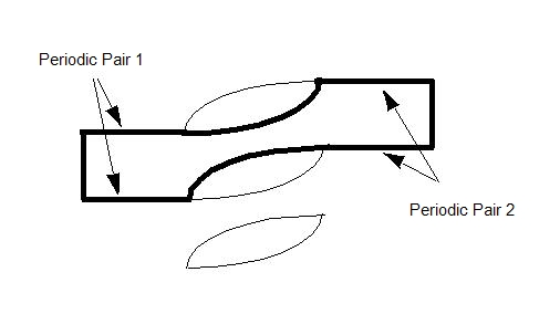
To assign a Periodic condition to Pair 1:
- Select the first surface of pair 1.
- Set the Pair ID to 1 and the Side ID to 1.
- Click Apply.
- Select the second surface of Pair 1.
- Set the Pair ID to 1 and Side ID to 2.
- Click Apply.
Repeat for the remaining pairs.
Periodic boundary conditions are a convenient way to include the effect of multiple repeating features in a simplified model. Because of the repeating geometry, the flow upstream and downstream of a device will be the same for each passage.