By default, particle traces are the path a particle without mass would take when released into the flow. A more physically real visualization technique is to include the effects of mass on the particle. The resulting trace behaves more like a physical substance within a flow system.
Inertial and drag effects are taken into account, and if a particle has too much inertia to turn a corner, it will hit the wall. Massed particles will bounce when they strike a wall or a symmetry surface. The coefficient of restitution can be specified to control the amount of bounce in a collision.
There are several settings that provide a great deal of flexibility for the visualization of massed particles. The most basic is the ability to select the particle density and particle radius. Other settings include a user-prescribed initial path, the inclusion of gravity, and a customizable drag correlation.
These features are located in the Mass dialog. Open this dialog by clicking the Mass button on the Particle Trace task dialog. Begin by checking Enable mass.
Massed particle traces are only drawn forward, not backward, so it is best to position the seed points near the inlet of the geometry.
Required Quantities and Units
Enter the Particle Density and Particle Radius, and select the desired units for both quantities. The default density is the fluid density, and the default radius is based on the bounding box of the model.
Coefficient of Restitution
This coefficient of restitution is a measure of the amount of bounce between two objects. Specifically, it is the ratio of the velocities of the objects before and after an impact, and can be described mathematically as:
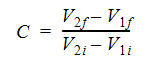
- V1 is the velocity of the first object
- V2 is the velocity of the second object
- i and f subscripts indicate initial and final velocity, respectively.
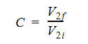
For massed particles, the other object is a static wall, so this equation reduces to:
The coefficient of restitution can range between 0.01 and 1:
- A value of 0.01 is an inelastic collision, and the particles stick when they hit the wall.
- A value of 1 is a perfectly elastic collision, and particles have the same velocity (and kinetic energy) after the collision as they did before.
- The default value is 0.5.
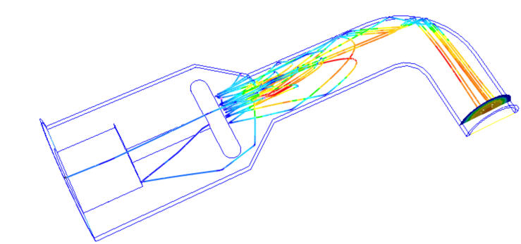
An example massed particles with a Coefficient of Restitution value of 0.01:
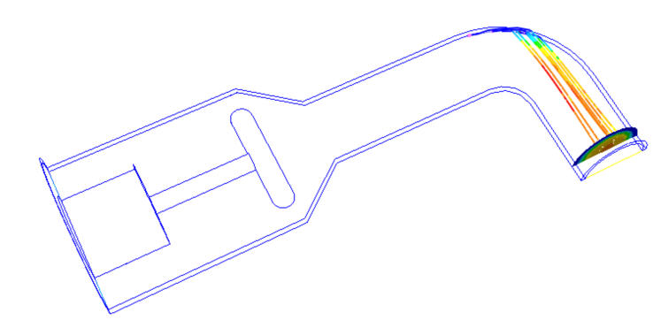
An example massed particles with a Coefficient of Restitution value of 1:
Initial Path
Specify an initial velocity and direction for the trace by checking Set Initial Velocity.
This allows the visualization of the interaction between the flow and a particle injection with a known velocity and trajectory. An example is an aerosol injection of particles into a flow stream.
Gravity
Include the effects of body forces on particle traces by checking the Enable Gravity for massed particles.
Enter the components of the force in the X, Y, and Z boxes.
For Earth’s gravity, check the Earth box, and enter a unit vector to indicate the direction in which gravity acts.
Modifiable Drag Correlation
The drag correlation used for massed particles is given as:
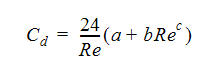
Modify the coefficients a, b, and c to change the drag as appropriate.
Erosion
激しい流れの環境で機器の故障を引き起す主要な原因の1つに、高速な流体流れの衝突によるサーフェスの腐食があります。腐食が発生する可能性がある箇所を把握することは、優れた耐久性と長いサービス寿命のための設計を行う上で重要です。
砂、クォーツ、飛散灰などの混入物質がバルブなどの機構で再循環し、衝突する際に、材料の腐食が生じます。石油およびガス産業では、エンジニアが粒子の「メッシュサイズ」に基づいてこの延性腐食を評価します。メッシュサイズは、システム内への混入が考えられる最大粒子サイズです。この現象は、「ウォッシュアウト」とも呼ばれます。
Autodesk® CFD では、Edwards Model を使用した Lagrangian 粒子追跡によって腐食を計算します。低い粒子集中度の想定(スラリー腐食モデルでない)を採用し、結果をスカラー結果量として提示します。これにより設計の比較が容易になり、腐食予測の解釈を当て推量で行うことがなくなります。
腐食モデルは仰角の反発データと材料のブリネル硬さを使用して材料ボリュームの除去率を計算します。このアプローチは、腐食の対象領域を質的に特定します。流れと腐食傾向の間の関係を明らかにすることで、設計を改良して腐食を軽減できます。
Time Step Size
As a particle passes through elements, the drag calculations are based on the local velocity field from one time step to the next. The velocity acting on the particle is computed using geometric weighting based on the velocity values at the node vertices of the element where the particle is currently traveling though. The distance that the particle travels in a time step is equal to its velocity multiplied by the time step size.
If the time step size is too large, the particle may travel through several elements in a single time step. This yields a coarse approximation to the actual motion, since the velocity fields within some of the intermediate elements that the particle passed through were not considered. The most accurate path will be computed when the time step size is approximately equal to the time required for the particle to pass through a single element. If the particle passes though a single element in a time step, then the local velocity field and drag estimates consider all the elements along the path. This yields the best accuracy.
It is good practice to reduce the time step size until the particle path is un-affected by reducing the time step size further.