Tutorial 21: To Adjust Mesh Settings for Simulation Utility LT

Work within the mesh complexity limits of Simulation Utility LT

Video length (5:01).

Sample files for use with the tutorials are available on the Download Page.

1. In Simulation Utility LT, click Simulation > Open.
2. Browse to your saved Example files folder, and open Example_21.tivus.
   
3. Open the Machine dialog and select the Ti-6Al-4V (250 W) option from the Processing parameters drop-down menu. This PRM file uses a generic set of processing conditions, common across a variety of powder bed fusion machines. Click OK to accept.
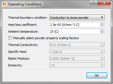
4. Open Operating Conditions and set Thermal boundary condition to Conduction to loose powder. Click OK.
   
5. Click Mesh Settings. Make sure the Meshing approach is set to Layer based. Change Coarsening generations to 0 and Layers per element to 5.
   

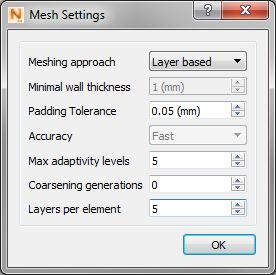
   This corresponds to the finest mesh settings recommended for use. Layers per element can be set lower than 5 for parts with very fine features that need to be captured, but is generally not recommended, and may frequently exceed the meshing limitations allowed by Simulation Utility LT.

6. Click OK to accept.

   A note about what these mesh settings mean:

   • Coarsening generations – This sets the number of allowable adaptive mesh coarsening levels from the finest element size. This is a powerful tool to drastically reduce the mesh density to represent a geometry in voxel form and speed up simulation time by grouping together smaller elements into larger elements. Simulation Utility LT is limited to the values of 0 and 1 coarsening generations.
   • Layers per element – This establishes the finest possible element size. The base element size is established by multiplying the powder bed thickness, saved in the PRM file, by the Layers per element. For this example, the Ti-6Al-4V PRM file has a 0.040 mm layer thickness and 5 layers are grouped, so the finest possible element size is 0.20 mm (5 layers X 0.04 mm). The larger the number of elements grouped together, the larger the base element is, and thus the coarser the overall mesh will be. Simulation Utility LT allows a maximum of 20 Layers per element.
7. Click Mesh Preview. This will take a few minutes to complete, because of the fine mesh settings.
8. Open the solver output by clicking the View Logs button on the Home tab. The logs are a text-based output of the solver that record the progress of the meshing of simulation, along with any errors or warnings that may occur, and information about the processing conditions, and base geometry.

   At the end of the meshing process, the log will report two Errors, indicating that the mesh exceeds the limitations of Simulation Utility LT. A notification will also pop up in the upper right corner of the window, showing the same error messages. After the error message disappears, you can press the bell icon in the upper right of the interface to show the errors for the current simulation. The following errors are shown:
   
   

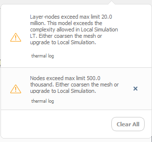
   • Layer-nodes exceed max limit of 20 million. A Layer-node is simply the number of layer groups X number of nodes of the final mesh.
   • Nodes exceed maximum limit of 500 thousand.
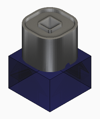
9. At the end of the Mesh Preview run, the resulting mesh appears.
   

   This mesh has 122 million layer-nodes and 957 thousand nodes, as recorded on the Mesh preview item in the Browser. You may see different values, but they far exceed what Simulation Utility LT can run.

   The example operating conditions and meshing choices used for our first mesh preview are extreme, beyond what is necessary to have a useful simulation of this model. These choices will be revisited to show how to get the model within the limitations of Simulation Utility LT.

10. Return to Operating Conditions and change the Thermal boundary conditions setting to Uniform heat loss.

    This setting changes the thermal boundary conditions on all surfaces of the model and base plate to a uniform heat loss value of 25 W/m °C. This value has been shown to give a good approximation of thermal losses into the surrounding powder. Using this boundary condition also significantly reduces the number of elements and nodes, as the powder elements are all removed, leaving just the component and base plate to be meshed.

11. Click OK to accept, and press Mesh Preview again to see if this brings the model within the acceptable meshing limits. Since a mesh already exists, a prompt will ask to overwrite those results. Click Yes to proceed.

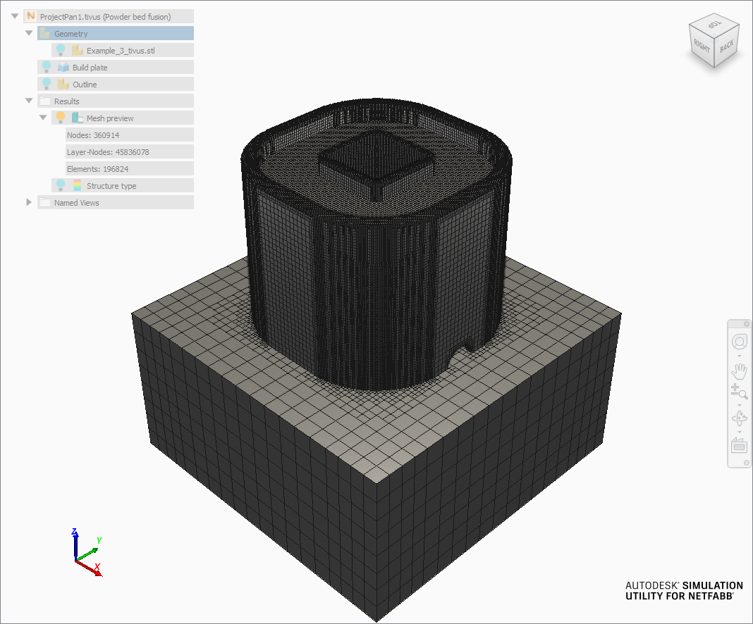
    The meshing operation should take far less time. However, the resulting mesh, as indicated by the pop up error notifications, is still too dense, with 46 million layer-nodes. The number of nodes has fallen within the allowable bounds at 361 thousand.
    
    

12. Return to the Mesh Settings dialog and set Coarsening generations to 1. Press OK to accept, and press Mesh Preview again to see if the new mesh setting brings the model within the acceptable meshing limits.
    

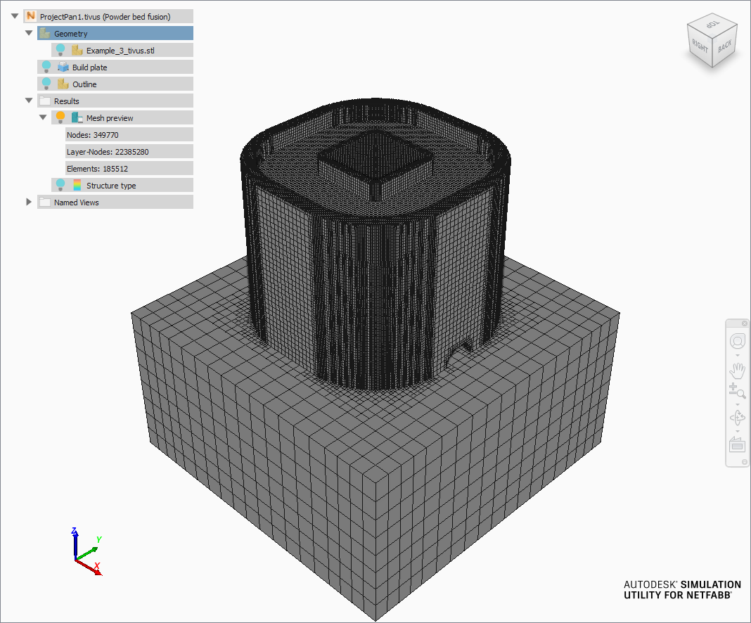
    The resulting mesh is just over the allowable bounds, with 22 Million layer-nodes.

13. Return to the Mesh Settings dialog again and change Layers per element to 6. Press OK to accept, and press Mesh Preview again to see if the new mesh setting brings the model within the acceptable meshing limits.
    

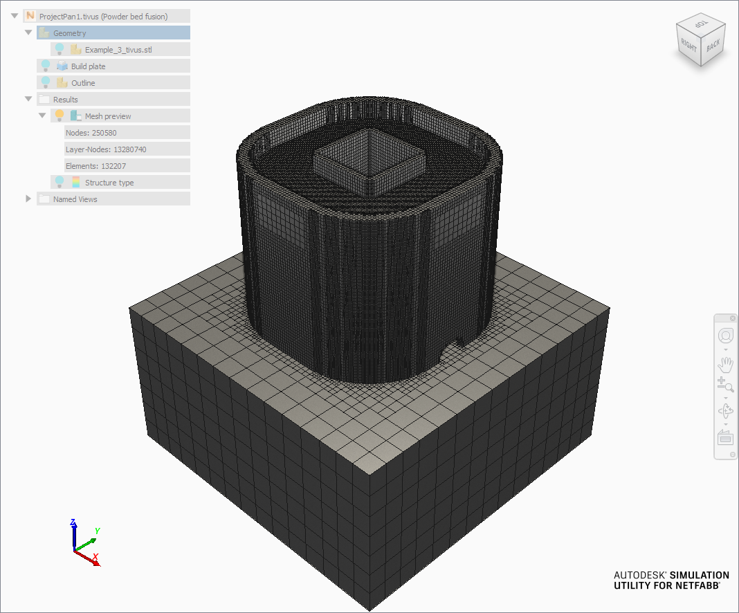
    Note upon meshing that neither the log file nor the error notification pop-up yield an Error. This set of operating conditions and mesh settings have brought the mesh settings within the bounds allowed by Simulation Utility LT, with 251 thousand nodes and 13 million layer-nodes. This geometry can now be solved to see how this component develops stress and distortion and various thermal effects using generic Ti-6Al-4V processing conditions.