Tutorial 19: To Scale a PRM File

Learn why and how to scale PRM files.

Video length (5:03).

Sample files for use with the tutorials are available on the Download Page.

This tutorial guides you through a scenario in which PRM scaling functionality can be used to improve simulation accuracy. For this exercise, assume that a test geometry has been printed out of Inconel 718. Experimental measurements show a peak distortion along the external face of 0.40 mm. This test print is used to validate the PRM file before more complex geometries will be simulated and optimized prior to printing.

1. Click Simulation menu > Open, browse to the sample folder Example_19, and open the model Example_19.tivus.

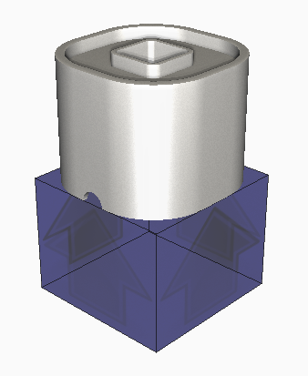
   This imports the STL file and automatically sizes the build plate:

   
2. Click Home tab > Machine to open the Machine dialog.
   
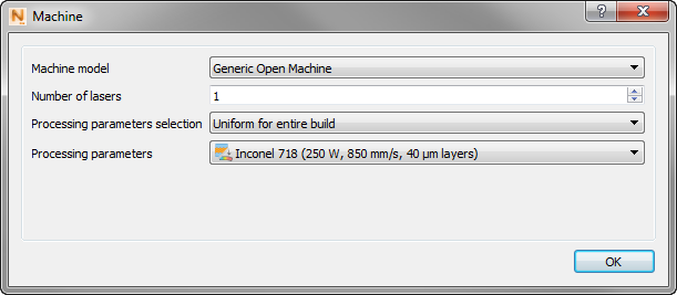
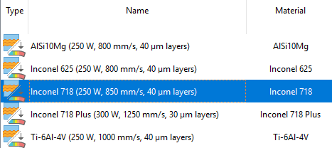
3. In Processing parameters, select the Inconel 718 PRM file.
   
4. Click Home tab > Build Plate.

   Deselect Match part deposition material, and in the Material menu, select SAE 304 stainless steel, which is commonly used with Inconel powder.

   
   
   
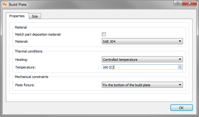
5. Under Thermal conditions, Heating, select Controlled temperature.
6. In the Temperature box type 160 (C).
7. Click OK.
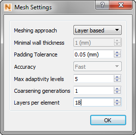
8. In Mesh Settings, change the Meshing approach to Layer based.
9. Change the Coarsening generations to 1 and the Layers per element to 18.
10. Click OK.
    
    
    
11. On the Home tab, click Solve to run the simulation.
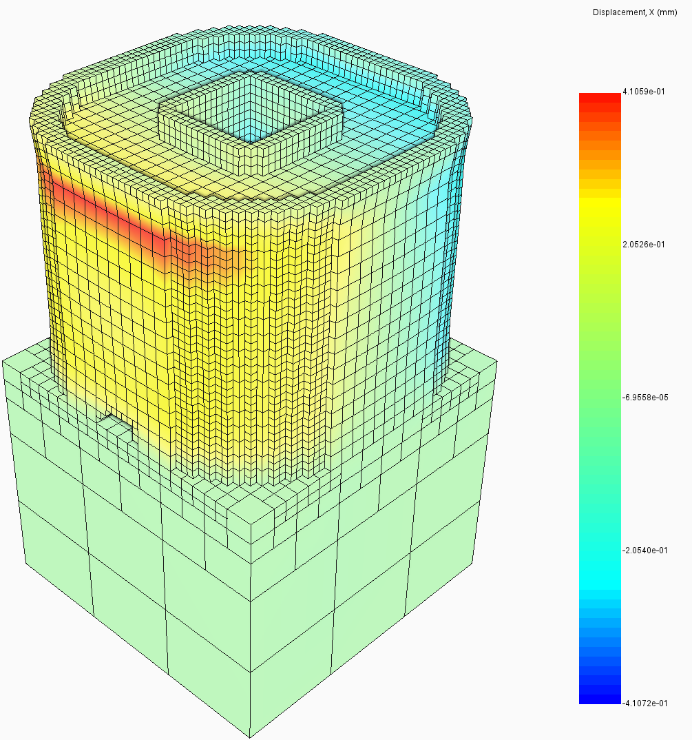
12. When the simulation finishes, the results are displayed and the Results tab opens.
13. To compare the displacements to experimental results, click Plot Settings .
    
    
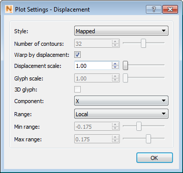
14. In the Component drop-down menu, change the value to X, then click OK.
    
    
    

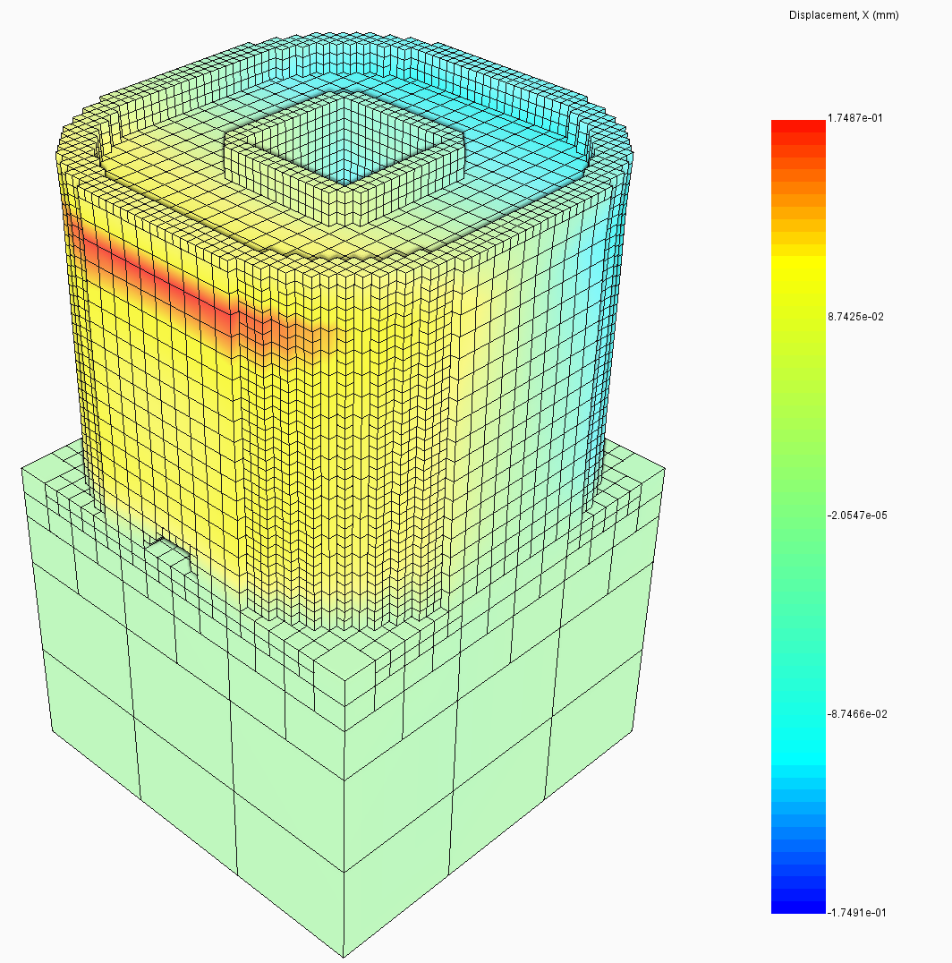
    The peak distortion predicted using the generic Inconel 718 PRM file is 0.17 mm which is much lower than the experimentally measured 0.40 mm. The model-measurement correlation can be improved by scaling the PRM file.

15. Return to the Home tab and open the Processing Parameters dialog.
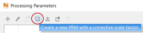
16. Select the generic Inconel 718 PRM file provided with Simulation Utility and click the scaling button, as shown below.
    
17. Assuming that the scaling for this part's distortion is linear, the Scale Factor should be the measured distortion divided by the predicted distortion, which in this case is 0.40 mm/0.17 mm = 2.35. Enter 2.35 into the Scale Factor box. Click OK.
    
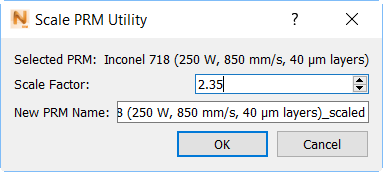
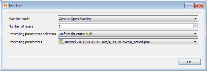
18. The scaled PRM file will be added to the Processing Parameter library, with _scaled appended to the name. To simulate the part with the scaled PRM, return to the Machine dialog. On the Processing parameters drop-down, select the newly scaled PRM file, which is probably last in the list.
    
    
19. Click Solve again. When prompted to overwrite previous results, select OK to proceed.
20. The new results are loaded.
    Remember: To see the correct displacement results, on the Results tab, click Plot Settings and set the Component value to X, as you did for the first simulation results.
    
    
    

    Using the scaled PRM file attains model results within 1% of the actual measurements. This scaled PRM file can then be used to perform simulations of this material and processing parameter combination with confidence in the accuracy of the predicted distortion.