Thermal analysis
From a command line run
$ pan -b 02_thermal
The -b option runs the solver in background mode, which automatically overwrites any previous results, and directs output to a an output file of the format input-file-name.out.
The analysis progress is written to file 02_thermal.out. To check progress on Linux, run
$ tail 02_thermal.out
To check progress in a Windows command line, run
$ type 02_thermal.out
After the analysis completes, the last few lines of the output file 02_thermal.out should be similar to the following:
Increment end
-----------------------------
CPU wall for increment 34 = 00:00:00.43, since start = 00:00:14.12
 inc =      35 time =     4249.1602     iter =    1 eps = 0.23990E+03
 inc =      35 time =     4249.1602     iter =    2 eps = 0.42313E-12
Finished writing file results\02_thermal_35.case
Writing record:           2, time      4249.16015625000
Increment end
CPU wall for increment 35 = 00:00:00.25, since start = 00:00:14.37
Layer end

Mesh preview volume  =   761.062500000000
Activated volume     =   761.062500000000
Activated percentage =   100.000000000000

Finished writing file .\02_thermal.case

Analysis completed

CPU wall for printing = 00:00:06.31
CPU wall  = 00:00:14.43
CPU total = 00:00:29.01

Peak RAM used for this process = 90,716 kB

END Autodesk Netfabb Local Simulation
Actual CPU times will differ from system to system.
Quasi-static mechanical analysis
Run the analysis from the command line:
$ pan -b 02_mechanical
The analysis progress is written to file 02_mechanical.out. To check progress on Linux, run
$ tail 02_mechanical.out
or in Windows run
$ type 02_mechanical.out
After the analysis completes, the last few lines of the output file 02_mechanical.out should be similar to the following:
----------------------------------
Substrate removal time increment
----------------------------------
 inc =       36 time =    6249.1602    iter =    1 eps =  0.53336E+04
 inc =       36 time =    6249.1602    iter =    2 eps =  0.10599E-08

Optimizing rigid body motion...
Initial RMS displacement          =      3.346287E-01
Optimized RMS displacement        =      3.179544E-01
Number of optimization iterations =          250
Rotation matrix =
    1.000000E+000 -9.670484E-006 -1.151088E-007
    9.670483E-006 1.000000E+000 -2.613098E-006
    1.151341E-007 2.613097E-006 1.000000E+000
Translation =    -2.369873E-005   1.993509E-004   1.043245E-001

Finished writing file results\02_mechanical_36_f.case
Finished writing file results\02_mechanical_36.case
Increment end
CPU wall for increment 36 = 00:00:00.81, since start = 00:00:23.51
Layer end

------------------------------------------------------
Total number of equilibrium iterations:      72

Mesh preview volume  = 761.062500000000
Activated volume     = 761.062500000000
Activated percentage = 100.000000000000

Finished writing file .\02_mechanical_f.case
Finished writing file .\02_mechanical.case

Analysis completed

CPU wall for substrate removal = 00:00:00.86
CPU wall = 00:00:23.57
CPU total = 00:01:03.33

Peak RAM used for this process = 337,664 kB

END Autodesk Netfabb Local Simulation
Actual CPU times will differ.
Results can be imported and viewed in the Simulation Utility for Netfabb or in ParaView. Figure 2 shows the computed final distortion after substrate release.
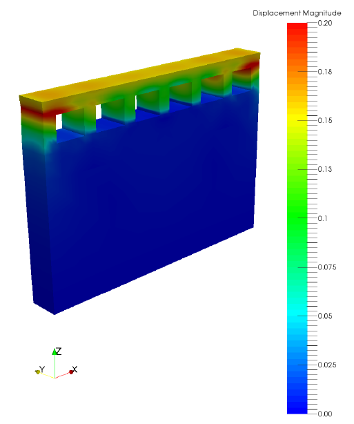
Figure 2: Final distortion
Producing distorted and compensated STL files from the simulation results
After the thermo-mechanical simulation is completed, the mechanical results can be used to output warped and compensated STL files. Warped STLs can be used for post-process analysis, to ensure assembly fit or other dimensional checks. To produce a warped STL, use the included program distort_stl.
$ distort_stl warp.txt
By default the program uses the distortion results after cool down but before removing the part from the build plate. The resulting distorted STL, 02_mechanical warp.STL, is shown in Figure 3.

Figure 3: Warped STL
A compensated STL takes the prediction distortion results, inverts them, and applies them to the original geometry. This produces a geometry which should distort into the desired shape. To produce the compensated geometry, use the distort_stl program again:
$ distort_stl comp.txt
The resulting compensated STL, 02_mechanical_compensated.STL, is shown in Figure 4.

Figure 4: Compensated STL