Exercise P14: Displaying Multispectral Imagery

In this exercise you combine several image bands from a multispectral dataset into a single displayed image.

While each band of a multispectral data set can be displayed individually as a grayscale image, the real analytic value of this data type is revealed when you assign two or three bands to different color channels and display them as a “false color” image.

In this exercise, you will use color map controls to display a set of seven image bands in different ways.

Related Exercises

• Exercise A2: Managing Images in a Drawing
• LiveView Exercise: Editing Color Maps in Getting Started, “Task-Specific Concepts”

Exercise

1. In the \Tutorial5 folder, open the drawing file Multispec_CA.dwg.

   This drawing contains a multispectral set of seven satellite images, and the color map is set to display a standard false color image.

2. If the Image Manager toolspace is not open, click RasterManage.

   Use a standard false color map

3. In Image Manager, expand the object tree under the drawing name so you can see the color map (R:B40 G:B30 B:B20), which is configured as follows:
   • Red channel – B40 (Visible Near Infrared)
   • Green channel – B30 (Red)
   • Blue channel – B20 (Green)

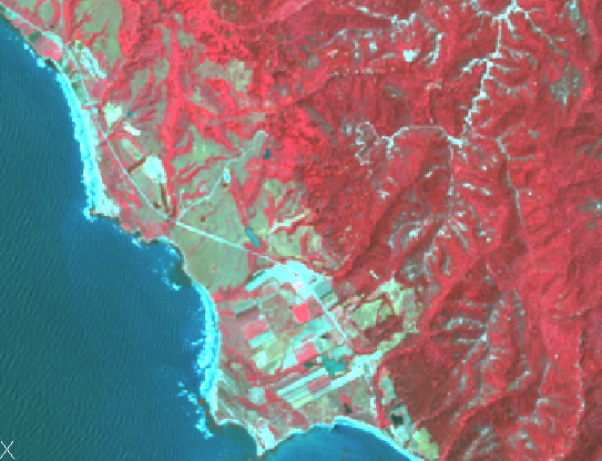
   This color map produces an image in which different types of vegetation and water are easier to see, so it is useful for analyzing water depths and land cover. In the next few steps we will look at two examples.

4. Click View menu Named Views. Then set the current view to Trees.

   In this view, coniferous forest cover is dark red, and deciduous forest cover is lighter red.

   
5. Click View menu Named Views. Then set the current view to Water.

   In this view, clear water is dark blue, and shallow or sedimented water is light blue. The underwater channels and shelves are clearly visible.

6. Click View menu Named Views. Then set the current view to Vegetation.

   Create a natural color map

7. In Image Manager, right-click the image color map, click Edit Color Map, and assign the color channels to image bands as follows:
   • Red channel – B30 (Red)
   • Green channel – B20 (Green)
   • Blue channel – B10 (Blue)

     This color map shows the terrain in colors close to its natural appearance. The gray urban area in the upper right is bordered by light brown hills with green forest cover. By changing color maps, we can see the features of this region in greater detail.

     Create a color map for analysis of land cover

8. In Image Manager, right-click the image color map, click Edit Color Map, and assign the color channels to image bands as follows:
   • Red channel – B40 (Visible Near Infrared)
   • Green channel – B50 (Mid Infrared)
   • Blue channel – B30 (Red)

     Band 5 (B50) is very sensitive to variations in moisture content of plants and ground surface. As a result, this color map shows varying amounts of green coloration for different types of land cover.

     

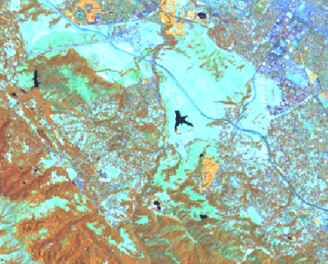
     In this view, trees are reddish brown, but drier vegetation has more green tones, so it appears orange or green. Natural grasslands in this photo are dry and sparsely covered, so they appear light greenish blue. Bare soil and urban areas appear blue and gray.

     Create a color map for analysis of rock and soil

9. In Image Manager, right-click the image color map, click Edit Color Map, and assign the color channels to image bands as follows:
   • Red channel – B70 (Far Infrared)
   • Green channel – B40 (Visible Near Infrared)
   • Blue channel – B20 (Green)

     Band 7 in this color map displays the moisture content of rocks and soils as shades of red, with darker red indicating more moisture. Because band 4 is assigned to the green channel, vegetation appears in different shades of green.

10. Close your drawing without saving changes.