To Select Dynamic Simulation Settings

Once you set these options, they effect Dynamic Simulation until you change them. Set options immediately after opening Dynamic Simulation.

1. On the ribbon, click Environments tab Begin Panel Dynamic Simulation to display the Dynamic Simulation panels.
2. Then click Dynamic Simulation tab Manage panel Simulation Settings .
3. Click Automatically Convert Constraints to Standard Joints to set the automatic Dynamic Simulation converter (Constraint Reduction Engine or CRE) to on.

   The default is on.

   When you click OK, the CRE automatically converts assembly constraints to standard joints and updates converted joints the next time you open this mechanism.

4. If you want to be warned when a mechanism is over-constrained, click Warn when mechanism is over-constrained.

   While this setting is the default for new mechanisms, it is not enabled by default for mechanisms created before version 2008. When you enable this option, if the mechanism is over-constrained, the software shows a message after you click OK and before it automatically creates the standard joints.

5. If you want a visual indication of the components included in the various mobile groups, check the Color Mobile Groups checkbox. Predefined color overrides are assigned to components in the same mobile group. This option aids in analyzing component relationships. To return the components to their normally assigned colors, clear the checkbox in the settings dialog box, or right click the Mobile Groups node and select Color Mobile Groups
6. Click All initial positions at 0,0 if you want to set all initial positions of the DOF to 0 without changing the actual position of the mechanism.

   It is useful for viewing variable plots starting at 0 in the Output Grapher.

7. Click Reset all to reset all coordinate systems to the initial positions given during joint coordinate system construction.

   This setting is the default.

8. Click AIP Stress Analysis to prepare all FEA information for analysis by AIP Stress Analysis.

   This function saves data relevant to FEA in the part files of parts you select.

9. Alternatively, click ANSYS Simulation to prepare a file containing all FEA information for export to ANSYS.

   This function saves data relevant to FEA in a file that ANSYS can read.

   • In the text entry box, enter the name of the file you want to hold FEA information for export to ANSYS.
   • Alternatively, click Save in to specify an existing file or create a file.

     If you select an existing file, the software overwrites all data currently in the file.

     Note: If using Ansys Workbench version 10 or 11, perform an additional file modification. Open the text file, locate the section entitled “Inertial State.” In this section, there are two lines that must be removed. The lines are “Grounded” and the associated code, either a “0” or “1” on the line that follows.
10. Click More to see more properties.
11. To show your copyright information on AVI files you generate, click Display a copyright in AVIs and enter your copyright information in the text entry box.
12. Click Input angular velocity in revolutions per minute (rpm) to enter angular speeds in rpms.

    The output, however, is in the units defined when you selected the empty assembly file.

13. To set the length of the assembly coordinate system Z axis for 3D frames in the graphics window, enter the percentage value in the Z axis size edit box.

    By default, the Z axis size is equal to 20% of the diagonal of the bounding box.

14. Click OK or Apply.

    Both save your settings, but OK also closes this dialog box.

Micro Mechanism Model

This option is designed to work with mechanisms having small mass properties.

In the standard mode, the calculation fails if mass or inertia is less than 1e-10 kg or 1e-16 kg.m2. The dynamic equations is then solved with a Gauss procedure with precision set to 1e-10 (below this value, pivot is set to 0).

When the Micro Mechanism Mode is activated, mass or inertia must be greater than 1e-20 kg and 1e-32 kg.m2. The Gauss precision is set to 1e-32.

To determine when to enable this option, check the mass properties provided in the joint coordinate system.

• If there is a translation degree of freedom, we check the mass.
• If there is a rotational degree of freedom along the X-axis, we check the principal inertia Ixx along the X axis, and not the cross inertias Ixz and Ixy as they are of no interest.

Example 1
For a mechanism where the smallest part has a mass m = 6.5e-9 kg and principal inertias Ixx = 1e-20 kg/m2, Iyy = 1e-20 kg.m2, even if Izz > inertia limit = 1e-10 kg.m2:
	If this part has only a rotational DOF along the Z axis, the MM mode is not necessary because Izz > inertia limit = 1.0e-10 kg.m2 If this part has only a translational DOF

Attention: Only activate the Micro Mechanism Mode when you are simulating a small mechanism. At the same time, you should modify Assembly Precision to optimize it for small parts. See Assembly Precision for more information.

Assembly Precision

Applicable to closed loop and 2D Contact cases only.

2D Contact: defines the maximum authorized distance between contact points. The default value is 1e-6m = 1μm.

• This distance is always checked at the end of Runge-Kutta steps.
• If the distance between these points does not exceed the assembly precision, positions and velocities are accepted, and the calculation continues with the integration error estimation .
• If the distance exceeds the assembly precision, positions are corrected until the distance does not exceed the assembly precision. Then, based on these new positions, velocities are corrected, and the calculation continues with the integration error estimation.

Closed Loop: same as 2D Contact, but can also have angular constraints (expressed in radians) based on the joint type.

• Distance and angular constraints are checked at the end of the Runge-Kutta steps.
• If distance constraints do not exceed the assembly precision, and angular constraints do not exceed the assembly precision multiplied by 1e3 (with assembly precision expressed in meters), positions and velocities are accepted, and the calculation continues with the integration error estimation .
• Otherwise, positions are corrected until distance constraints do not exceed the assembly precision and angular constraints do not exceed the assembly precision multiplied by 1e3. Velocities are then corrected, and the calculation continues with the integration error estimation.

Modifying Assembly Precision

The Assembly Precision parameter can be modified in the following situations:

• The mechanism cannot be assembled at the beginning or during the simulation. First, check the feasibility of your mechanism (is the requested position realistic and can it be reached by the mechanism. Check imposed motions that can lead to contradictory positions). If no problem is detected and if the scale of your mechanism is large (in the order of 1 m), then increase the assembly precision (1e-5m or 1e-4m). If the scale is small (less than 10 mm), then decrease the assembly precision (1e-7m or 1e-8m).
• In cases where the mechanism is smaller than 1 mm, decrease the assembly precision (1e-8m to 1e-10m) or use the Micro Mechanism Model.

Attention: Do not impose an assembly precision less than 1e-12. It does not add value and can cause simulation problems.

Solver Precision

Dynamic equations are integrated using a five order Runge-Kutta integration scheme. The integration error and time step, in order to guarantee acceptance, are managed as follows:

• At the end of each Runge-Kutta step, based on the calculated velocities and accelerations, the integration error is estimated.
• This integration error is compared to the user-defined parameter “solver precision”.
• If the integration error does not exceed the solver precision, the step is accepted and the integration continues.
• If the integration error exceeds the solver precision, the step is rejected. A new time step, smaller than the actual time step, is then calculated and the simulation is restarted from the beginning of the step with the new time step value.

The integration error is estimated using certain properties of the Runge-Kutta formulas. It allows easy calculation of the positions “p” and velocities “v” to fifth order (vectors noted “p5” and “v5” respectively) and fourth order (vectors noted “p4” and “v4”). The integration error is then defined on positions and velocities as follows:

Integ_error_position = norm(p5 - p4) Integ_error_velocity = norm(v5 - v4) Where norm denotes a special norm.

When a step is accepted, the following relationships exist (in metric units):

Integ_error_position = norm(p5 - p4) < Atol + | p5 | . Rtol Integ_error_velocity = norm(v5 - v4) < Atol + | v5 | . Rtol

With:

	Atol	Rtol
Translational degree of freedom	Solver precision Default = 1e-6 No maximum value	Solver precision Default = 1e-6 No maximum value
Rotational degree of freedom	Solver precision . 1e3 Default = 1e-3 Maximum value = 1e-2	Solver precision . 1e3 Default = 1e-3 Maximum value = 1e-2

To illustrate this process, consider the following examples:

Example 1: Illustrate a relative error Rtol
Joint type: Slider joint 1 with position and velocity
	p[1] = 4529.289768 m v[1] = 18.45687455 m/s
If the solver precision is set to 1e-6 (default), results to six digits are guaranteed:
	p[1] = 4529.28 m v[1] = 18.4568 m/s
If the solver precision is set to 1e-8, eight digits are guaranteed:
	p[1] = 4529.2897 m v[1] = 18.456874 m/s
Example 2: Illustrate a relative error for Atol
Joint type: Slider joint 1with position and velocity
	p[1] = 0.000024557 m v[1] = 0.005896476 m/s
If the solver precision is set to 1e-6 (default), results to six digits after the decimal point are guaranteed:
	p[1] = 0.000024 m v[1] = 0.005896 m/s
If the solver precision is set to 1e-8, eight digits after the decimal point are guaranteed:
	p[1] = 0.00002455 m v[1] = 0.00589647 m/s
The same reasoning is valid with a pin joint, but with Atol and Rtol having equal solver precision multiplied by 1e3:
Example 3: Illustrate a relative error for Rtol
Joint type: Pin joint 2 with position and velocity
	p[2] = 12.53214221 rad v[2] = 21.36589547 rad/s
If the solver precision is set to 1e-6 (default), results to three digits is guaranteed:
	p[2] = 12.5 rad v[2] = 21.3 rad/s
If the solver precision is set to 1e-8, five digits are guaranteed:
	p[2] = 12.532 rad v[2] = 21.365 rad/s

The Solver Precision parameter can be modified in the following cases:

• The simulation stops with an error message and the time step is small enough to guarantee a good quality result. If you have small displacements, decrease solver precision. If you have large displacements, increase solver precision.
• When 2D contacts are activated (status = 1). If you have small forces, decrease the solver precision. If you have large forces, increase solver precision. It is not valid for forces at shock instants.
• When working with small mechanisms (less than 1 mm). In such cases, decrease the solver precision or check Micro Mechanism Model option.

Attention: Solver precision is directly linked to time step size. Do not decrease solver precision too much (for example, less than 1e-12). Doing so significantly affects simulation time.

Capture Velocity

This parameter is used for simulating impact between objects. It helps the solver to limit the number of small bounces before constant contact results. The shock model uses a restitution coefficient “e”. The value is specified by the user, and is from 0 through 1. For the resulting conditions, the values are treated as follows:

• When e = 0, there is maximum energy dissipation. For example, take the case of a simple ball falling on a plane, from an initial height with no initial velocity and under gravity effect, there is no observable bounce, the contact status = 1.
• When e = 1, there is no energy dissipation. Using the ball example, the ball bounces returning to its initial position, the contact status = 0.5. The movement is periodic and continues infinitely.
• When e>0 and e<1, there is energy dissipation at each impact. Using the ball example again, it will bounce, but the bounce height decreases after each impact and reaching the limit, the ball rests on the plane, at which point the contact status = 1. For this set of conditions, the capture velocity is operative.

The Capture Velocity parameter helps the solver limit the number of small bounces that occur before contact is considered active or constant. The capture process is as follows:

• Impact is calculated with all restitution coefficients set to their initial values.
• Post-impact relative velocities, which represent lift-off velocities, are compared to the capture velocity parameter for all contacts.
• If all relative velocities are greater than the capture velocity or null, the impact is accepted and the solver advances in time using the new velocities as initial parameters.
• If on relative velocity is less than the capture velocity and not null, e = 0 is imposed for that contact to maximize energy loss and the impact is calculated again. If the impact is accepted, all restitution coefficients are reset to their initial values.

Attention: Contact status (e = 1) is never programmatically imposed. The solver manages contact status so that all active contacts are coherent. The solver determines it with a non-linear quadratic equation.

When can the parameter be modified?

This parameter can be modified in the following case:

• When you have 2D contacts and the simulation is slow. Stop the simulation, plot the Capture Velocity. If the parameter is varying at each time step (varies between 0 - 1 - 2) or is equal to 1, there is a capture issue. The solver is trying to stabilize the status of your contacts, but it takes time and is complex. In this situation, increase the capture velocity.
• There is no benefit derived by reducing the parameter value.

Regularization Velocity

In 2D contacts, a real non-linear Coulomb friction law is used. In joints and 3D contacts, for simplicity and to avoid a hyperstatic condition, a regularized Coulomb law is used, and can be illustrated as follows:

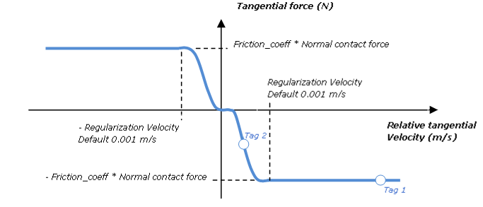
Regularization is driven by the velocity regularization parameter.

Using this model, in cases of sticking contact (or rolling contact), when the relative tangential velocity equals zero, the tangential force is null.

In the case of joint friction in a rotational degree of freedom, the tangential force is replaced by a tangential torque (unit: Nm) and the tangential relative velocity is a rotational velocity (unit: rad/s), both are calculated by multiplying the tangential force and dividing the translational velocity by the joint radius.

Example 1
A pin joint with a radius of 10 mm is piloted with a constant velocity “w” equal to 10 rad/s. We apply a force (Fn) equal to 20 N to the joint, perpendicular to its rotation axis, and the friction coefficient (mu) is set to 0.1. In this case, the friction torque (Uf) in the joint can be calculated as follows:
	? = r * w = 0.01 * 10 = 0.1 m/s ? > regularization velocity = 0.001 m/s => Uf = -mu * r * Fn = -0.1 * 0.01 * 20 = -0.02 Nm See “tag 1” in the regularized Coulomb graph.
Example 2
Using the same example, but with a velocity (w) of 0.05 rad/s, the friction torque (Uf) is then given by:
	? = r * w = 0.01 * 0.05 = 0.0005 m/sm ? > regularization velocity = 0.001 m/s => Uf ≈ -mu * r * Fn/2 = -0.1 * 0.01 * 20/2 = -0.01 Nm See “tag 2” in the regularized Coulomb graph.

The Regularization Velocity parameter can be modified in the following situations:

• Your simulation is slow and you have small oscillations on a joint with friction or in a 3D contact joint. The friction in the joint or 3D contact creates a significant stiffness in your model, so the solver is decreasing the time step to maintain reliable precision. You must decrease the stiffness => increase the regularization velocity parameter by a factor of 5 (5e-3 m/s). If the model is still slow, you can continue increasing the parameter using values relative to your model (lower in comparison to the velocities in your model).
• Do not increase the regularization velocity significantly, otherwise it will only work between these values. The friction force will never reach its maximum value. This results in artificially limiting the friction effect.

Numerical validation

Before analyzing simulation results, it is important to check that your simulation is numerically valid, which means it is insensitive to numerical parameters. To perform the numerical validation step do the following:

1. Run a simulation with a set of numerical parameters (solver and assembly precision, capture velocity, regularization velocity, and time step), then save it.
2. For each parameter, divide the parameter by 10, run the simulation, and save it.
3. Plot all the results on the same graph. If all your results are close, your simulation is then insensitive to numerical parameters. Otherwise, there is a sensitivity issue.
4. If the simulation is insensitive, the results can be analyzed.
5. If the simulation is sensitive to numerical parameters, using the result curves, determine which numerical parameter is the causing the sensitivity. Divide the parameter by 10 and take the resulting value as a nominal value for the numerical parameter. Restart the validation from the beginning. To save time, you can validate insensitivity for the one parameter.