Described here are the governing thermal equations solved by the Simulation Utility, along with the formulation of the thermal boundary conditions required to resolve the temperature field throughout the history of the deposition process.
Thermal equilibrium
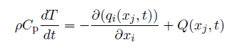
Equation 2
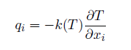
Equation 3
To solve these equations it is necessary to have an initial condition, a heat input model, and thermal boundary conditions. The initial condition for the first time step is to set the temperature to either the ambient or preheating temperature for the substrate or build plate elements. For subsequent time steps the initial condition are the nodal temperatures calculated at the previous time step. In the following section, the thermal boundary conditions and their numeric implementation are described.
The heat input model
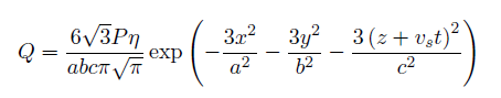
Equation 4
where P is the power, η is the absorption efficiency; x, y, and z are the local coordinates; a, b, and c are the transverse, melt pool depth, and longitudinal dimensions of the ellipsoid respectively, vs is the heat source travel speed, and t is the time.
Boundary losses
During AM process heat losses may occur due to thermal radiation, free convection, forced convection, or conduction through fixturing bodies.Convection
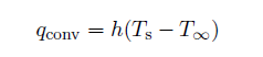
Equation 5
where qconv is the convective heat flux, h is the heat transfer coefficient, and Ts is the surface temperature.
Radiation
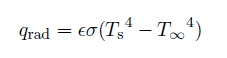
Equation 6
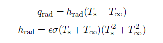
Equations 7 and 8