Results may be imported and viewed in Simulation Utility for Netfabb or ParaView.
Moving adaptivity thermal analysis
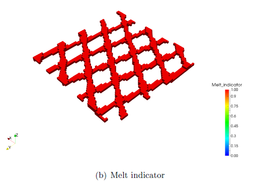
Figure 1 shows the results of the two state variables added to the ParaView results when using *LFUS in the moving adaptivity simulation.

Figure 1: *LFUS results moving adaptive mesh, (a) Peak temperatures
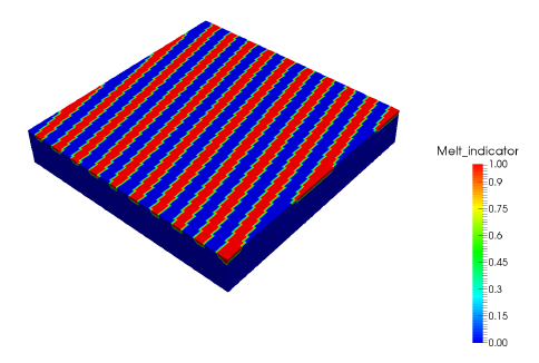
(b) Melt indicator
Using *TPRE in this simulation also produces a file t10_moving_tpre.txt, which gives the increment time, heat source location, preheat temperature at that heat source location, and binary flags (1 for those that exceed the test temperatures, 0 for those that fall below) for the temperatures of interest.
*TPRE results file t10_moving_tpre.txt
These are the results for the first 40 time increments:
# time, laser_x, laser_y, laser_z, Temp_start, StateVar1 for Temp_crit = 6.900000E+02, 1.600000E+03,
# time, laser_x, laser_y, laser_z, Temp_start, StateVar1 for Temp_crit = 6.900000E+02, 1.600000E+03,
2.110243E-04, 9.812045E-01, 6.025919E-02, 0.000000E+00, 1.183370E+03, 1, 0,
2.110243E-04, 9.812045E-01, 6.025919E-02, 0.000000E+00, 1.183370E+03, 1, 0,
2.310243E-04, 9.616060E-01, 5.627184E-02, 0.000000E+00, 1.246882E+03, 1, 0,
2.310243E-04, 9.616060E-01, 5.627184E-02, 0.000000E+00, 1.246882E+03, 1, 0,
2.510243E-04, 9.420075E-01, 5.228448E-02, 0.000000E+00, 1.264094E+03, 1, 0,
2.510243E-04, 9.420075E-01, 5.228448E-02, 0.000000E+00, 1.264094E+03, 1, 0,
2.710243E-04, 9.224090E-01, 4.829712E-02, 0.000000E+00, 1.249736E+03, 1, 0,
2.710243E-04, 9.224090E-01, 4.829712E-02, 0.000000E+00, 1.249736E+03, 1, 0,
2.910243E-04, 9.028105E-01, 4.430976E-02, 0.000000E+00, 1.274152E+03, 1, 0,
2.910243E-04, 9.028105E-01, 4.430976E-02, 0.000000E+00, 1.274152E+03, 1, 0,
3.110243E-04, 8.832120E-01, 4.032240E-02, 0.000000E+00, 1.260694E+03, 1, 0,
3.110243E-04, 8.832120E-01, 4.032240E-02, 0.000000E+00, 1.260694E+03, 1, 0,
3.310243E-04, 8.636136E-01, 3.633504E-02, 0.000000E+00, 1.281517E+03, 1, 0,
3.310243E-04, 8.636136E-01, 3.633504E-02, 0.000000E+00, 1.281517E+03, 1, 0,
3.510243E-04, 8.440151E-01, 3.234769E-02, 0.000000E+00, 1.262331E+03, 1, 0,
3.510243E-04, 8.440151E-01, 3.234769E-02, 0.000000E+00, 1.262331E+03, 1, 0,
3.710243E-04, 8.244166E-01, 2.836033E-02, 0.000000E+00, 1.269745E+03, 1, 0,
3.710243E-04, 8.244166E-01, 2.836033E-02, 0.000000E+00, 1.269745E+03, 1, 0,
3.910243E-04, 8.048181E-01, 2.437297E-02, 0.000000E+00, 1.275913E+03, 1, 0,
3.910243E-04, 8.048181E-01, 2.437297E-02, 0.000000E+00, 1.275913E+03, 1, 0,
4.110243E-04, 7.852196E-01, 2.038561E-02, 0.000000E+00, 1.293645E+03, 1, 0,
4.110243E-04, 7.852196E-01, 2.038561E-02, 0.000000E+00, 1.293645E+03, 1, 0,
4.310243E-04, 7.656211E-01, 1.639825E-02, 0.000000E+00, 1.322355E+03, 1, 0,
4.310243E-04, 7.656211E-01, 1.639825E-02, 0.000000E+00, 1.322355E+03, 1, 0,
4.510243E-04, 7.460226E-01, 1.241089E-02, 0.000000E+00, 1.332978E+03, 1, 0,
4.510243E-04, 7.460226E-01, 1.241089E-02, 0.000000E+00, 1.332978E+03, 1, 0,
4.710243E-04, 7.264241E-01, 8.423535E-03, 0.000000E+00, 1.375219E+03, 1, 0,
4.710243E-04, 7.264241E-01, 8.423535E-03, 0.000000E+00, 1.375219E+03, 1, 0,
4.910243E-04, 7.068256E-01, 4.436177E-03, 0.000000E+00, 1.396394E+03, 1, 0,
4.910243E-04, 7.068256E-01, 4.436177E-03, 0.000000E+00, 1.396394E+03, 1, 0,
5.110243E-04, 6.872271E-01, 4.488181E-04, 0.000000E+00, 1.405183E+03, 1, 0,
5.110243E-04, 6.872271E-01, 4.488181E-04, 0.000000E+00, 1.405183E+03, 1, 0,
1.033910E-03, 2.024131E-01, 3.860940E-03, 0.000000E+00, 1.218541E+03, 1, 0,
1.033910E-03, 2.024131E-01, 3.860940E-03, 0.000000E+00, 1.218541E+03, 1, 0,
1.053910E-03, 2.220116E-01, 7.848298E-03, 0.000000E+00, 1.281124E+03, 1, 0,
1.053910E-03, 2.220116E-01, 7.848298E-03, 0.000000E+00, 1.281124E+03, 1, 0,
1.073910E-03, 2.416101E-01, 1.183566E-02, 0.000000E+00, 1.294444E+03, 1, 0,
1.073910E-03, 2.416101E-01, 1.183566E-02, 0.000000E+00, 1.294444E+03, 1, 0,
1.093910E-03, 2.612086E-01, 1.582301E-02, 0.000000E+00, 1.300685E+03, 1, 0,
1.093910E-03, 2.612086E-01, 1.582301E-02, 0.000000E+00, 1.300685E+03, 1, 0,
These preheating results can also be visualized using the visual tool of the user’s choice (e.g. Scilab, Matlab, Python). An example for a similar simulation using a 3 mm × 3 mm block is presented in Figure 2.

Figure 2: Visualization of *TPRE results, (a) Colorbar
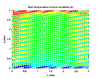
(b) *TPRE Contour
Multilayer thermal analysis
Figure 3 shows the results of the two state variables added to the ParaView results when using *LFUS in the multilayer adaptive simulation. ParaView has a filter option Threshold that will show only those elements with values within a specified range for scalar results, which makes it easier just to investigate the region of melt.
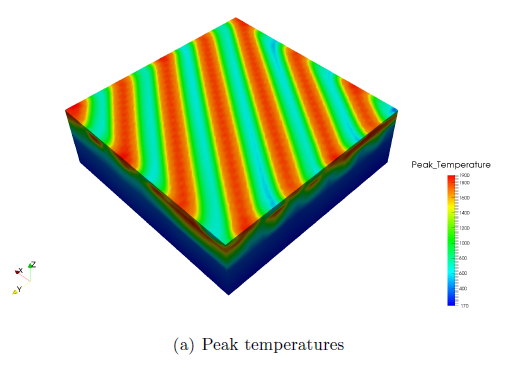
Figure 3: LFUS results multilayer mesh
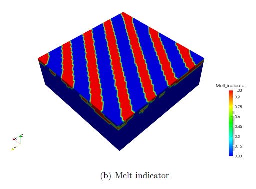
Figure 4 shows the peak temperature and melt indicator results for elements that have a melt indicator value of 1.
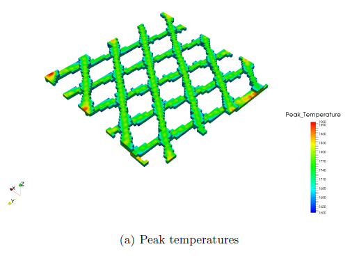
Figure 4: LFUS results multilayer mesh using threshold filtering
Using *TPRE in this simulation also produces a file t10multilayer_tpre.txt, which gives the increment time, heat source location, preheat temperature at that heat source location, and binary flags (1 for those that exceed the test temperatures, 0 for those which fall below) for the temperatures of interest.
*TPRE results file t10multilayer_tpre.txt
These are the results for the first 40 time increments:
# time, laser_x, laser_y, laser_z, Temp_start, StateVar1 for Temp_crit = 6.900000E+02, 1.600000E+03,
2.110243E-04, 4.812045E-01, 6.025919E-02, 0.000000E+00, 9.967262E+02, 1, 0,
2.110243E-04, 4.812045E-01, 6.025919E-02, 0.000000E+00, 9.967262E+02, 1, 0,
2.310243E-04, 4.616060E-01, 5.627184E-02, 0.000000E+00, 1.047308E+03, 1, 0,
2.310243E-04, 4.616060E-01, 5.627184E-02, 0.000000E+00, 1.047308E+03, 1, 0,
2.510243E-04, 4.420075E-01, 5.228448E-02, 0.000000E+00, 1.064964E+03, 1, 0,
2.510243E-04, 4.420075E-01, 5.228448E-02, 0.000000E+00, 1.064964E+03, 1, 0,
2.710243E-04, 4.224090E-01, 4.829712E-02, 0.000000E+00, 1.062888E+03, 1, 0,
2.710243E-04, 4.224090E-01, 4.829712E-02, 0.000000E+00, 1.062888E+03, 1, 0,
2.910243E-04, 4.028105E-01, 4.430976E-02, 0.000000E+00, 1.068414E+03, 1, 0,
2.910243E-04, 4.028105E-01, 4.430976E-02, 0.000000E+00, 1.068414E+03, 1, 0,
3.110243E-04, 3.832120E-01, 4.032240E-02, 0.000000E+00, 1.065790E+03, 1, 0,
3.110243E-04, 3.832120E-01, 4.032240E-02, 0.000000E+00, 1.065790E+03, 1, 0,
3.310243E-04, 3.636136E-01, 3.633504E-02, 0.000000E+00, 1.069138E+03, 1, 0,
3.310243E-04, 3.636136E-01, 3.633504E-02, 0.000000E+00, 1.069138E+03, 1, 0,
3.510243E-04, 3.440151E-01, 3.234768E-02, 0.000000E+00, 1.070207E+03, 1, 0,
3.510243E-04, 3.440151E-01, 3.234768E-02, 0.000000E+00, 1.070207E+03, 1, 0,
3.710243E-04, 3.244166E-01, 2.836032E-02, 0.000000E+00, 1.074631E+03, 1, 0,
3.710243E-04, 3.244166E-01, 2.836032E-02, 0.000000E+00, 1.074631E+03, 1, 0,
3.910243E-04, 3.048181E-01, 2.437297E-02, 0.000000E+00, 1.081879E+03, 1, 0,
3.910243E-04, 3.048181E-01, 2.437297E-02, 0.000000E+00, 1.081879E+03, 1, 0,
4.110243E-04, 2.852196E-01, 2.038561E-02, 0.000000E+00, 1.089785E+03, 1, 0,
4.110243E-04, 2.852196E-01, 2.038561E-02, 0.000000E+00, 1.089785E+03, 1, 0,
4.310243E-04, 2.656211E-01, 1.639825E-02, 0.000000E+00, 1.109395E+03, 1, 0,
4.310243E-04, 2.656211E-01, 1.639825E-02, 0.000000E+00, 1.109395E+03, 1, 0,
4.510243E-04, 2.460226E-01, 1.241089E-02, 0.000000E+00, 1.128674E+03, 1, 0,
4.510243E-04, 2.460226E-01, 1.241089E-02, 0.000000E+00, 1.128674E+03, 1, 0,
4.710243E-04, 2.264241E-01, 8.423532E-03, 0.000000E+00, 1.158016E+03, 1, 0,
4.710243E-04, 2.264241E-01, 8.423532E-03, 0.000000E+00, 1.158016E+03, 1, 0,
4.910243E-04, 2.068256E-01, 4.436173E-03, 0.000000E+00, 1.179002E+03, 1, 0,
4.910243E-04, 2.068256E-01, 4.436173E-03, 0.000000E+00, 1.179002E+03, 1, 0,
5.110243E-04, 1.872271E-01, 4.488143E-04, 0.000000E+00, 1.182956E+03, 1, 0,
5.110243E-04, 1.872271E-01, 4.488143E-04, 0.000000E+00, 1.182956E+03, 1, 0,
8.739096E-04, 1.879548E-02, 6.822967E-02, 0.000000E+00, 1.008571E+03, 1, 0,
8.739096E-04, 1.879548E-02, 6.822967E-02, 0.000000E+00, 1.008571E+03, 1, 0,
8.939096E-04, 3.839398E-02, 7.221703E-02, 0.000000E+00, 1.062931E+03, 1, 0,
8.939096E-04, 3.839398E-02, 7.221703E-02, 0.000000E+00, 1.062931E+03, 1, 0,
9.139096E-04, 5.799247E-02, 7.620439E-02, 0.000000E+00, 1.084469E+03, 1, 0,
9.139096E-04, 5.799247E-02, 7.620439E-02, 0.000000E+00, 1.084469E+03, 1, 0,
9.339096E-04, 7.759097E-02, 8.019175E-02, 0.000000E+00, 1.089238E+03, 1, 0,
9.339096E-04, 7.759097E-02, 8.019175E-02, 0.000000E+00, 1.089238E+03, 1, 0,
Using timex for multilayer adaptivity simulations
From the command line run
$ timex timex-madap-input.txt
This is similar to the timex input file shown in Example 1, but with the additional cards *CRSE and *SHFT which enable timex to work with multilayer adaptivity. The above example timex input file records the temperatures at the center of the build cross section x=0.25 mm, y=0.25 at 6 different z locations. Running the above command will produce the file timex_peaktemp_t10multilayer.txt. A plot of the temperatures at 6 queried locations is shown in Figure 5.
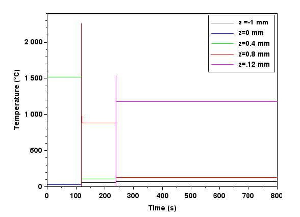
Figure 5: Multilayer adaptivity thermal history of the build region center at 6 z locations