View and Interpret Results

Examine the results of the progressive fatigue analysis.

Now that you have completed the progressive fatigue analysis using Helius PFA, the focus of the discussion will be centered around viewing and interpreting results. Viewing results from a progressive fatigue simulation is very similar to viewing results from a traditional Helius PFA static progressive failure analysis. The meanings of the solution-dependent variables are modified for fatigue analyses, with the new meanings specified in the .mct file accompanying the completed analysis. Refer to the Helius PFA User's Guide for further details of each solution-dependent variable (Progressive Fatigue Results and Appendix C).

After the job has completed, start ANSYS APDL and open Tutorial_4.db. Click General Postproc > Data & File Opts and select Tutorial_4.rst. Click General Postproc > Read Results > Last Set to read the last set of results.

1. Since we are interested in SVAR2, type PLNSOL,SVAR,2 into the command prompt.

2. To view the true deformation scale, click PlotCtrls > Style > Displacement Scaling. Select the 1.0 (true scale) radio button in the dialog box that appears and click OK.

3. The plot should be similar to the plot shown below.

   

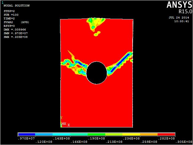
   The plot of SDV2 depicts the cycles to failure for each element. In the same manner that SVAR2 was plotted, a plot of SVAR1 can be made which will show the damage state of the model to verify that failure has occurred. You can also use nodal displacements and the cycles to failure for unfailed regions of the model reported in the Tutorial_4.txt file to create a plot of cycles to global structural failure as seen below.

   

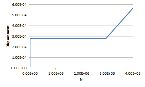   Note: At approximately 3.0E+06 cycles, the coupon begins to deform excessively, indicating the structure has failed catastrophically.