Tutorial B8: Set Up and Run the Analysis

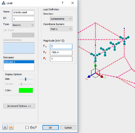
Apply the Load

The load is applied as a gravity load on the surface of the bolt hole.

1. Copy the following text:

   strCmdForLoad = "<Load Name=""Gravity Load"" ID=""1"" Type=""3"" SubType="""" EntitiesCount=""1"" Subcases=""1"" ArrowLength=""50"" ArrowColor=""65280"" DisplayDensity=""4"" Direction=""0"" CoordinateSystemID=""0"" Display=""1"" Fx=""0.0[N]"" Fy=""-9.81456[N]"" Fz=""0.0[N]"" HasVariableLoad=""0"" HasHeatGenTable=""0"" HadConvCoeffTable=""0"" HasRadTable=""0"" HasTransTable=""0"" HasVelTransTable=""0"" HasAccTransTable=""0"" HasVelFreqTable=""0"" HasAccFreqTable=""0"" HasFreqTable=""0"" HasFreqPhaseTable=""0"" HasAccFreqPhaseTable=""0""><Entity1 GeometryType=""0"" GeometryID="""" ComponentName=""Tutorial 2""/></Load>"

   Type = 3 denotes the use of a gravity load. GeometryType = 0 denotes that the load is applied on all the vertices of Subcase 1.

   These commands are equivalent to applying the load with the user interface.

   
2. Paste the text below the existing commands in the Edit Rule dialog.
3. Press the Enter or Return key twice to jump down to a new line.

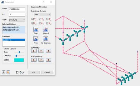
Apply the Constraint

The structure is constrained using a fixed boundary condition.

1. Copy the following text:

   strCmdForConstraint = "<Constraint Name=""Fixed Beams"" ID=""1"" Type=""0"" CoordinateSystemID=""0"" Tx=""1"" Ty=""1"" Tz=""1"" Rx=""1"" Ry=""1"" Rz=""1"" EntitiesCount=""2"" ArrowLength=""50"" ArrowColor=""14803200"" DisplayDensity=""4"" SubcaseCount=""1"" Subcases=""1""><Entity2 GeometryType=""3"" GeometryID=""42"" ComponentName=""Tutorial 2""/><Entity1 GeometryType=""3"" GeometryID=""30""/></Constraint>"

   Type = 0 denotes the use of a structural constraint. Each component (Tx, Ty, Tz, Rx, Ry, Rz) is defined with a value of 1, denoting a fixed boundary condition. GeometryType = 3 denotes that the boundary condition is applied on the two sketch entities with ID’s of 42 and 30.

   These commands are equivalent to applying the constraint with the user interface.

   
2. Paste the text below the existing commands in the Edit Rule dialog.
3. Press the Enter or Return key twice to jump down to a new line.

Solve the Model

Now that the model is defined, we can add the iLogic command that will solve the model.

1. Copy the following text:

   strCmdForSolve = "<RunAnalysis/>"

2. Paste the text below the existing commands in the Edit Rule dialog.
3. Press the Enter or Return key twice to jump down to a new line.