You will first run the nonlinear steady state heat transfer analysis to get the temperature distribution. This data will be input for a linear static analysis, which will be used for thermal stress analysis.
Set Up the Analysis
- In the tree view, right-click on Analysis 1 and choose Edit.
- Type Manifold Analysis for Name, and NL SS Heat Transfer for Title. Select Nonlinear Steady State Heat Transfer from the Type drop-down menu.
- The dialog should look as shown below.
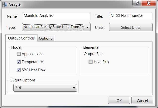
- Click OK to finish setting up the analysis and return to the tree view.
- In the Model tree, right-click on Materials and choose New.
- Change the Name to 4130 Alloy Steel.
- Make sure Thermal is selected, then enter 40.53 for C (Specific Heat) and 0.00055555 for K (Thermal Conductivity).
- Then under General enter 150 for TREF (Reference Temperature).
- Under
Structural, enter the properties shown in the image below. They will be used in the Linear Static Thermal Stress Analysis.
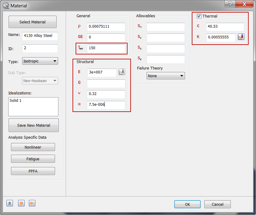
 With heat transfer analysis, the important material properties (thermal conductivity and specific heat) can be input under the
Thermal section. The mass density (
With heat transfer analysis, the important material properties (thermal conductivity and specific heat) can be input under the
Thermal section. The mass density ( ) can be input under the
General section. There is no need to input any structural properties.
) can be input under the
General section. There is no need to input any structural properties.
- Click OK.
- In the
Model tree, under
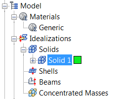
Idealizations, check for any existing definitions under the standard categories, such as
Solids and
Shells. Solid 1, shown below, is an example of an existing definition:
If there are any existing definitions, right-click . Doing this ensures that you won't have unwanted materials appearing in the part mesh and participating in the analysis.
- In the Model tree, right-click on Idealizations and select New.
- Type
Linear Solid Property for
Name, select
Solid Elements under
Type, and select
4130 Alloy Steel under
Material.
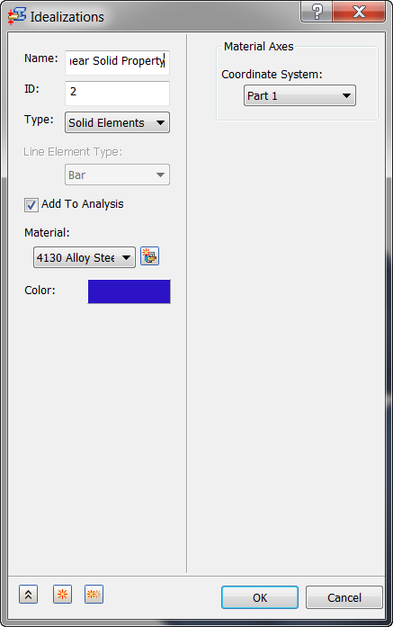
- Click OK.
Define the Mesh and Apply the Loads
- Right-click on Mesh Model and choose Edit.
- Type 0.09 in the Element Size field.
- Select
Linear from the
Element Order drop-down. Linear elements are good for thermal analysis.
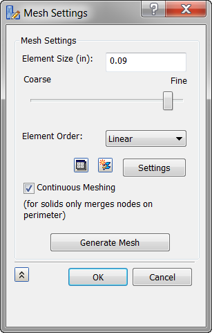 You are using linear solid elements because there is no need for midside nodes in heat transfer analysis.
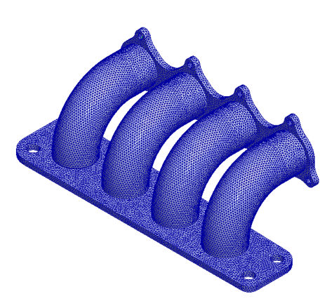
- Click OK.
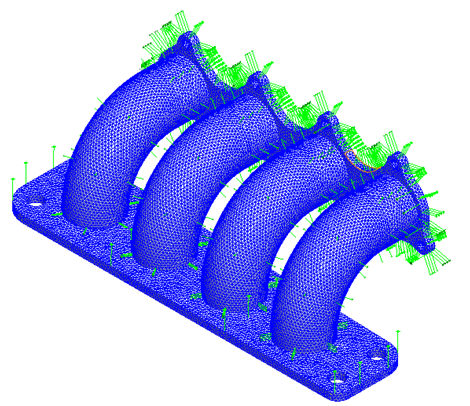
- After the mesh is generated, the model should look as shown below.
- Right-click on Loads under Subcase 1 and choose New.
- Enter NLssht Loads under Name.
- Select
Heat Flux from the
Type drop-down menu and select the inside surfaces for Flange 2 and all four tubes that make up the hole. The surfaces are highlighted in blue in the image below.
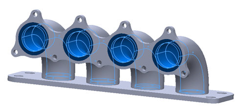
- Under
Load Definition enter
0.035 for
Heat Flux and make sure that
Subcase 1 is highlighted so that the load is automatically added to
Subcase 1.

- Click
 New button to define another load.
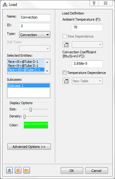
- Enter Convection under Name.
- Select Convection from the Type drop-down menu.
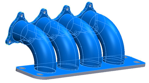
- Select one of the sides that make up the thickness of Flange 2 and select all the tangent surfaces to the surfaces already selected. Continue to select the surfaces of Flange 1 and 2 facing the tubes, as well as the exterior surfaces of the tubes. The surfaces that should be selected are shown below.
- Enter a Convection Coefficient value of 3.858E-5 BTU / (sec·in2·°F) and an Ambient Temperature of 70 °F.
- Make sure that
Subcase 1 is highlighted so that the load is automatically added to
Subcase 1.
- Click
New to define another load.
- When the Load dialog appears again, enter Initial Temperature in the Name field and select Initial Condition from the Type drop-down menu. Temperature should appear in the Sub Type drop-down. Then enter 70 under Temperature in the Load Definition section. This defines the initial temperature of the body and you are assuming that it is the temperature of the ambient air surrounding it.
- Select
Subcase 1 so that this load is automatically added to
Subcase 1.
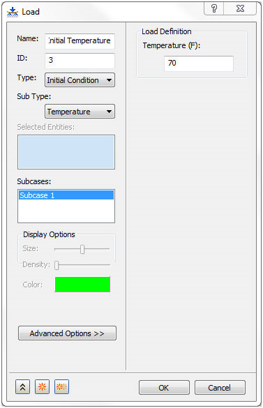
- Click OK.
- Save the model at this point.
Run the Analysis and Post-Process the Results
- Right-click on Manifold Analysis in the tree view and choose Solve in Nastran.
- When you see the dialog "Nastran Solution Complete", click OK to load the results into Inventor Nastran.
- Double-click on
Results. The
Plot dialog opens up.
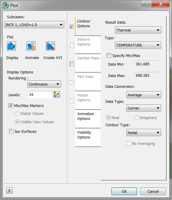
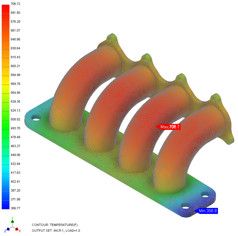
- Click
Display. The results should look as shown below.