The concept behind the moving solids modeling is rather simple. We assume that the fluid that comes in contact with a solid will take on the instantaneous velocity at the point of contact. In other words, we are applying a no-slip boundary condition in this situation.

For example, in the sketch below, a projectile is moving 100 mm per second from left to right. This means that the fluid along the surface of the solid will be assigned the 100 mm/s velocity at each time step.

To allow for arbitrary motion, a local coordinate system is placed within each moving part. It is assumed that the part does not move with respect to this local coordinate system. Rather, the local coordinate system moves relative to the global coordinate system.

The global coordinates of any point (x,y,z) on the moving part can be computed using the following transform.

where, (x, y, z) are the global coordinates computed at any time (t).

• are the coordinates of the moving part as viewed within the local coordinate system. They are marked with a superscript o to indicate that there are computed only once at time zero. By definition, they are time invariant.
• are the components of the local x axis.
• are the components of the local y axis.
• are the components of the local z axis.
• are the global position of the local coordinate system origin.

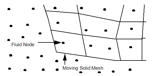
Rather than making a new mesh at each time level, the solid mesh is allowed to pass right through the fluid mesh. When a fluid node is “masked” by a solid element, then the velocity of the closest solid node is applied to this masked fluid node. In our diagram, the fluid node marked with the arrow is being masked by the solid element which is at the corner of the moving part. All the fluid nodes within the boundaries of the moving are considered “masked” and as such have their velocities controlled by the moving solid.

When models are initially constructed, many times these moving solids are embedded within the fluid. When the solid starts moving, we need a fluid region to appear in the area that the solid vacates. To handle this situation, all solids that are constructed such that they are in contact with the fluid, will have fluid elements and nodes automatically added. We refer to this action as replication. When models are constructed such that the moving solids are outside the fluid region, then no replication will take place.

Linear Motion

Linear motion is described along a given direction as shown in the figure below

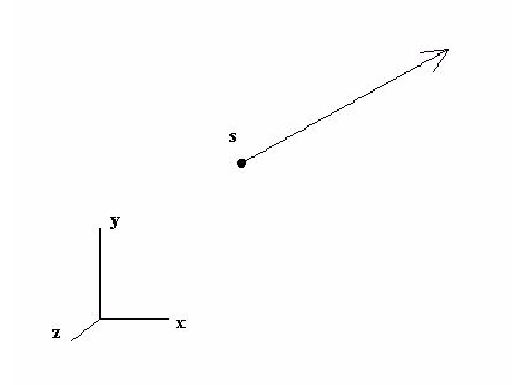
The displacement (denoted as s) is measured relative to the objects starting position. The user can define s as a function of time to move the object along the trajectory path. The trajectory is defined using a directional unit vector (Ux, Uy, Uz). The motion as defined in the global coordinate system is:

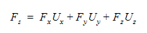
If the linear motion is flow-induced, then the shear and pressure forces as computed in the global reference frame are applied in the s direction using a dot product:

To this force, we can add prescribed forces and a spring force The equations of motion are:

where a is the acceleration, M is the mass, v is the velocity, s is the displacement and t is time.

Rotational Motion

For rotational motion, we have an object that rotates around an axis as shown in the figure below.

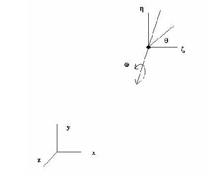
The axis about which the object rotates is defined using a unit vector (Ux, Uy, Uz). The center of rotation is given at a point (Px, Py, Pz). Angular measurement is made via the variable .

It is measured relative to the starting position of the moving object. In the local coordinate system, the motion can be described using versus time.

For a three-dimensional representation, it is convenient to represent the motion using directional cosines:

where:

If the motion is flow-induced, then the torque acting about the rotational axis is computed via a dot product:

User prescribed torque can be added to this torque as well. The equations of motion are:

where is the angular acceleration, Iu is the rotational inertia about the rotational vector, is the angular velocity, is the angular position and t represents time.

Combined Linear and Rotational Motion

If we combine the results of the two previous sections, then a combined motion can be described. The center of rotation will now translate as defined along the path given by s. The rotation will again be described locally, and the directional cosines globally. If the linear translation is flow induced, then the fluid forces will develop a force vector along the direction of travel and linear acceleration will result.

For flow-induced rotations, developed torques will be used to compute angular accelerations. If both motions are flow induced, it is assumed that the two motions are uncoupled and work independently to produce the overall motion. The linear translation equations will update the center of rotation over time and the rotation equations will update the directional cosines over time thus yielding a combined motion.

Orbiting and Rotational Motion

Orbiting motion involves an object moving in a circular path over time. The situation is shown in the figure below.

The variable is the radius or eccentricity of the orbit. It is computed using the point O and the point R:

Here, we have subtracted off the non-perpendicular vector to yield the perpendicular distance between the origin of the orbiting system and the axis of the rotating system. The vector (Ux, Uy, Uz) is a unit vector that described the axis of rotation for the orbiting system.

In a local coordinate system, the orbit is given by:

This can be expressed in the global reference frame by constructing a rotational transformation matrix as follows:

1. The local z axis () is equated with the orbiting axis U.
2. The local x axis () is constructed as the unit vector pointing from the origin of the orbiting system to the time=0 rotation system origin.
3. The local y axis () is constructed via crossing the local z axis with the local x axis.
4. Once all the local axes have been defined, a Gram-Schmidt procedure is undertaken to guarantee that this local system is truly orthogonal.

The global orbiting position as a function of can be written as:

If the orbiting motion is flow-induced, then forces acting on the moving object are summed and appropriate accelerations computed. Velocities and displacements are limited to the circular orbital path using the following relationships:

The orbiting equations of motion define the translation of the moving object. An object can also rotate as well at the point pointed to by the eccentricity vector. The rotation equations that were developed earlier govern this motion.

Nutating Motion

Nutating motion can be described using the figure below.

The precession or nutation angle is defined as . The angle defines the angular travel around the local z axis. The local y axis ( defines a position where a stop will permit motion in the local y and z planes (i.e.,=0 ). In local space, the directional cosines are:

As before, a rotation transformation matrix is used to create directional cosines in the global space.

If the nutating motion is flow-induced, the net torque is used to compute the angular accelerations in the same fashion as it was done for the rotating body discussed earlier.

Free Motion

This type of motion uses the unconstrained rigid body dynamics formulation described here.