General Scalar Transport Equation
The following equation describes the transport of a passive scalar through an incompressible fluid:

The variables in this equation are defined in the following table:
| Variable | Description |
| D | diffusivity (length2/sec) |
| f | passive scalar |
| t | time (sec) |
| u | velocity component in x direction (length/sec) |
| v | velocity component in y direction (length/sec) |
| w | velocity component in z direction (length/sec) |
In Autodesk® CFD, the species diffusivity (D) is entered on the Solve > Advanced dialog. The units of diffusivity are length squared divided by time (e.g., m2/sec).
For turbulent flow, the above equation is time-averaged, assuming the scalar variable can be represented as a superposition of a mean value and a fluctuating value, where the fluctuation is about the mean value. For example, the scalar variable can be written as:

where F is the mean scalar value and f"" is the fluctuation about this mean value. This representation is substituted into the governing equation and the equation is averaged over time. Using the notation that capital letters represent the mean values and lower case letters represent fluctuating values, the averaged turbulent scalar equation can be written as:

Note that the averaging process has produced extra terms in the scalar equation:  uf, vf and wf. These terms are combinations of fluctuating quantities resulting from averaging the non-linear inertia or advection terms.
Now a method must be found to “model” these extra terms, i.e. relate them back to the previous unknowns - mean values. At the zeroth level of closure, the extra terms are linked back to the dependent variable, F.
We will use the same level of closure as for the momentum equations, employing the Boussinesq approximation which defines an eddy diffusivity as:

If these definitions are used in the averaged scalar equation, the result is:

This leaves only the eddy diffusivity, D*t***, to be determined.
The eddy diffusivity is calculated using the eddy viscosity and the turbulent Schmidt number,  :
:

The turbulent Schmidt number is usually taken to be 1.0.
Boundary Conditions
There are 6 types of boundaries for which conditions must be imposed on the scalar equation: inlets, outlets, no-slip walls, symmetry lines, slip walls and periodic boundaries. For inlets, the value of the scalar should be specified, even if the value is zero. At outlets, symmetry lines, slip and no-slip walls the scalar equation uses a natural boundary condition of a zero gradient normal to the boundary. At periodic boundaries, the scalar at one boundary is enforced or translated to the corresponding point on the other periodic boundary.
Simulating Combustion Using the General Scalar
The scalar transport equation can be used to crudely simulate combustion. There are three processes which can limit the rate at which combustion proceeds:
- Macro-mixing - The large eddies of fuel and oxidant combine or interact by the action of convective and diffusive transport mechanisms.
- Micro-mixing - A molecule of fuel comes into contact with a molecule of oxidant.
- Chemical kinetics - The actual chemical process of the fuel reacting with the oxidant is governed by a set of chemical reactions which include several intermediate species. The rate of these reaction is determined by the species present and the local temperature.
Whichever of these processes has the slowest rate will largely determine the progress of the combustion process. A combustion process whose rate is constrained by either of 1 or 2 is said to be “mixing-limited”. In this case, we assume: “If it’s mixed, it’s burnt”. For this mixing-limited case, fuel and oxidant are assumed to always react in the stoichiometric proportions to form the major products of combustion. Intermediate species are ignored. For example, the stoichiometric reaction for a general fuel can be written:

where  is the stoichiometric coefficient required to burn 1 unit mass of fuel.
The fuel and oxidant can be combined into a single scalar variable:

 is the mass fraction of the fuel, i.e., the mass of the fuel divided by the total mass of the fuel plus oxidant.
 is the mass fraction of the oxidant.
This scalar variable becomes a conserved quantity, i.e., advective and diffusive transport balance in a steady-state calculation (no source or sink terms).
The transport equation for  is derived by subtracting times the oxidant species transport equation from the fuel species transport equation assuming equal exchange coefficients (diffusivities):

In this equation, the first term is the advection term and the second is the diffusive term. Using this newly defined scalar variable, we can define a mixture fraction as:

 is the value of the scalar in the fuel inlet stream
 is the value of the scalar in the oxidant inlet stream
With this definition of mixture fraction, the value of f in the fuel stream is 1.0 and 0.0 in the oxidant stream.
The value of f at stoichiometric conditions will be noted as f*st***.
Since f is a linear combination of values, it follows that f is also a conserved quantity. Hence, we can write the transport equation for f as:

Assuming equilibrium chemistry when the fuel and oxidant meet, the mass fraction of fuel and oxidant can be calculated:

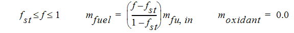
The mass fraction of the products can be determined from the remainders of these two equations.