Massed Particle Traces

By default, particle traces are the path a particle without mass would take when released into the flow. A more physically real visualization technique is to include the effects of mass on the particle. The resulting trace behaves more like a physical substance within a flow system.

Inertial and drag effects are taken into account, and if a particle has too much inertia to turn a corner, it will hit the wall. Massed particles will bounce when they strike a wall or a symmetry surface. The coefficient of restitution can be specified to control the amount of bounce in a collision.

There are several settings that provide a great deal of flexibility for the visualization of massed particles. The most basic is the ability to select the particle density and particle radius. Other settings include a user-prescribed initial path, the inclusion of gravity, and a customizable drag correlation.

These features are located in the Mass dialog. Open this dialog by clicking the Mass button on the Particle Trace task dialog. Begin by checking Enable mass.

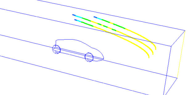
Massed particle traces are only drawn forward, not backward, so it is best to position the seed points near the inlet of the geometry.

Required Quantities and Units

Enter the Particle Density and Particle Radius, and select the desired units for both quantities. The default density is the fluid density, and the default radius is based on the bounding box of the model.

Note: Particle Radius values must be between 1e-12 and (the longest dimension of the part bounding box)/5. If you specify values outside of this range, the Particle Radius resets to the default value.

Coefficient of Restitution

This coefficient of restitution is a measure of the amount of bounce between two objects. Specifically, it is the ratio of the velocities of the objects before and after an impact, and can be described mathematically as:

coefficient of rest equation

V1 is the velocity of the first object
V2 is the velocity of the second object
i and f subscripts indicate initial and final velocity, respectively.

For massed particles, the other object is a static wall, so this equation reduces to:

coeff of restitution

The coefficient of restitution can range between 0.01 and 1:

A value of 0.01 is an inelastic collision, and the particles stick when they hit the wall.
A value of 1 is a perfectly elastic collision, and particles have the same velocity (and kinetic energy) after the collision as they did before.
The default value is 0.5.

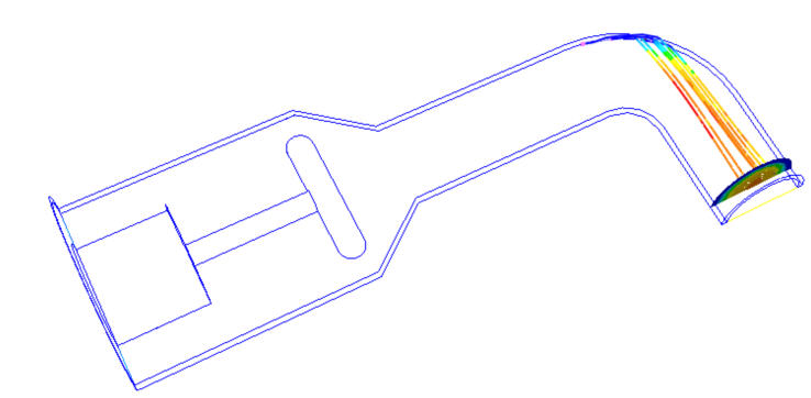
An example massed particles with a Coefficient of Restitution value of 0.01:

example low value

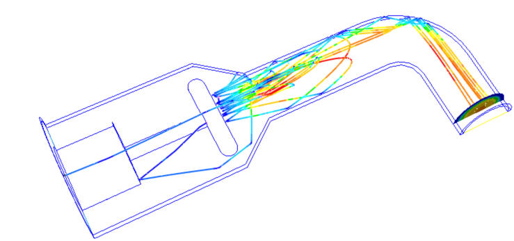
An example massed particles with a Coefficient of Restitution value of 1:

example high value

Initial Path

Specify an initial velocity and direction for the trace by checking Set Initial Velocity.

mass initial path

This allows the visualization of the interaction between the flow and a particle injection with a known velocity and trajectory. An example is an aerosol injection of particles into a flow stream.

Gravity

Include the effects of body forces on particle traces by checking the Enable Gravity for massed particles.

Enter the components of the force in the X, Y, and Z boxes.

For Earth’s gravity, check the Earth box, and enter a unit vector to indicate the direction in which gravity acts.

Modifiable Drag Correlation

The drag correlation used for massed particles is given as:

mass drag correlation

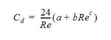
Modify the coefficients a, b, and c to change the drag as appropriate.

Erosion

One of the leading causes of equipment failure in harsh flow environments is surface erosion due to high-velocity liquid flow impingement. Understanding where erosion may occur is essential for designing for greater durability and longer service life.

Contaminants such as sand, quartz, and fly ash cause material erosion as they recirculate and impinge against valves and other machinery. In the oil and gas industry, engineers evaluate this Ductile erosion based on the "mesh size" of the particle. The mesh size is the largest particle size that is likely to be found in a system. This phenomenon is also referred to as "washout."

Autodesk® CFD uses Lagrangian particle tracking with the Edwards Model to compute erosion. A low particle concentration assumption (not a slurry erosion model) is employed, and results are presented as a scalar result quantity. This facilitates design comparison, and removes the guesswork from interpreting erosion predictions.

The erosion model uses angle of attack bounce data and the Brinell material hardness to compute the material volume removal rate. This approach qualitatively identifies areas subject to erosion. It illustrates the relationship between the flow and erosion trends, which can lead to erosion reduction through design improvements.

For more about computing erosion...

Time Step Size

As a particle passes through elements, the drag calculations are based on the local velocity field from one time step to the next. The velocity acting on the particle is computed using geometric weighting based on the velocity values at the node vertices of the element where the particle is currently traveling though. The distance that the particle travels in a time step is equal to its velocity multiplied by the time step size.

If the time step size is too large, the particle may travel through several elements in a single time step. This yields a coarse approximation to the actual motion, since the velocity fields within some of the intermediate elements that the particle passed through were not considered. The most accurate path will be computed when the time step size is approximately equal to the time required for the particle to pass through a single element. If the particle passes though a single element in a time step, then the local velocity field and drag estimates consider all the elements along the path. This yields the best accuracy.

It is good practice to reduce the time step size until the particle path is un-affected by reducing the time step size further.