Load variation is based upon a scalar surface. This allows three dimensional load variation. The variation has linear and quadratic distance weighted formulation so the distribution may not be exactly identical, but the load distribution will be very close. The use of the quadratic/parabolic distance weighted formulation allows less data points to be used for a “better” distribution.
This will be available in the Load form when you click on the Advanced Options button.
-
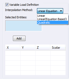
Interpolation Method:
- Linear: It interpolates using any two end points or vertices of the selected associated geometry in case of edge or curves. Four points are required in case of faces in order to interpolate the loads in linear order.
- Linear (Equation Based): It interpolates using any two end points or vertices of the selected associated geometry in case of edge or curves. Three points are required in case of faces in order to interpolate the loads in linear order using standard plane equation.
- Quadratic: It interpolates using any two end points or vertices of the selected associated geometry in case of edge or curves. Four points are required in case of faces in order to interpolate the loads in parabolic order.
-
Example 1: Simple 2D Variation on Flat Surfaces
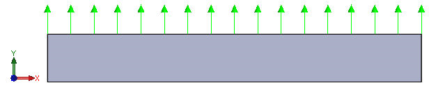
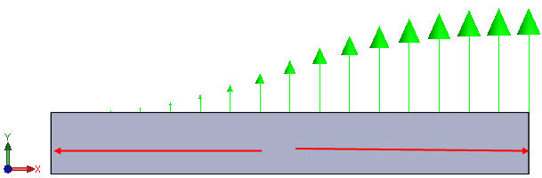
Consider a plate to which you want to apply a distributed load as shown in the images below.
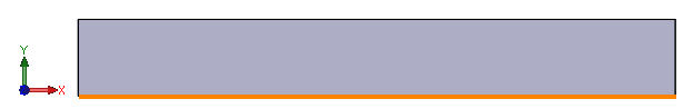
Define a unit load along the edge.
Check the Variable Load Definition box. Points and vertices may be used as Selected Entities, so it may be beneficial to create reference geometry when creating a variable load distribution for future models.
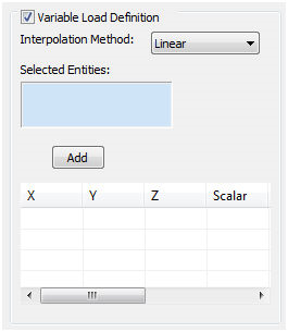
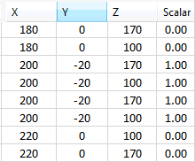
- Set the interpolation method as Linear. Select the two end points of the geometry using the Selected Entities selection box. It may be activated by clicking on it first.
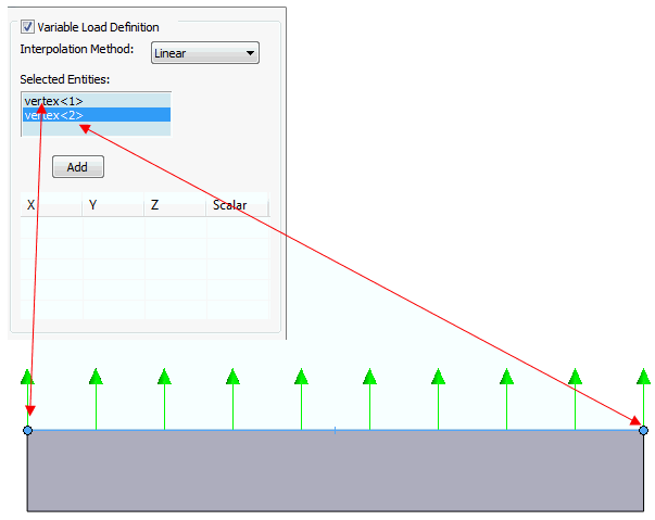
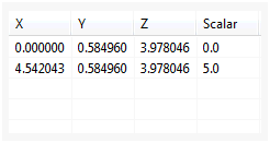
Click the Add button to add the three dimensional locations to the table.
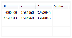
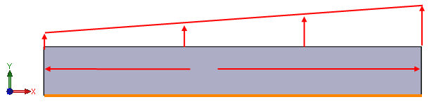
The first point has a scalar value of 0.0 and the second point has a scalar value of 5.0. Double-click in the Scalar boxes to enter a value.
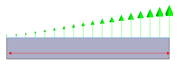
Notice that the curve is not a perfect linear curve, but parabolic. Based upon the dimensions above, it can be verified that the total load is 2.5.
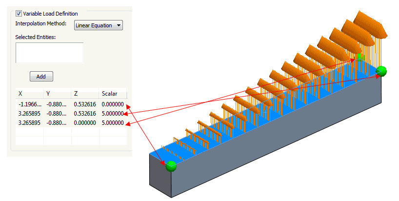
- Now change the interpolation method to Linear (Equation Based).
Notice that you will not be able to see the load arrows as the third point is missing for the surface. Select the third point and add it to the list and enter the same value of 5.0 as shown in the image below.
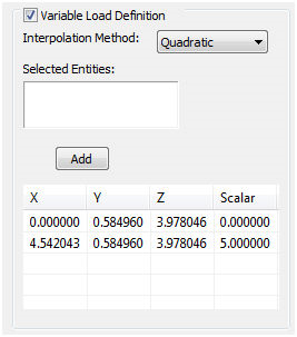
- Now change the interpolation method to Quadratic.
- Set the interpolation method as Linear. Select the two end points of the geometry using the Selected Entities selection box. It may be activated by clicking on it first.
-
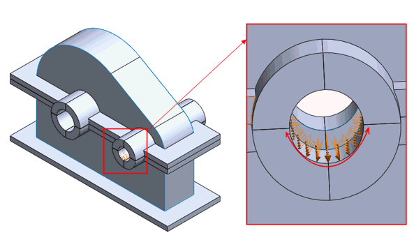
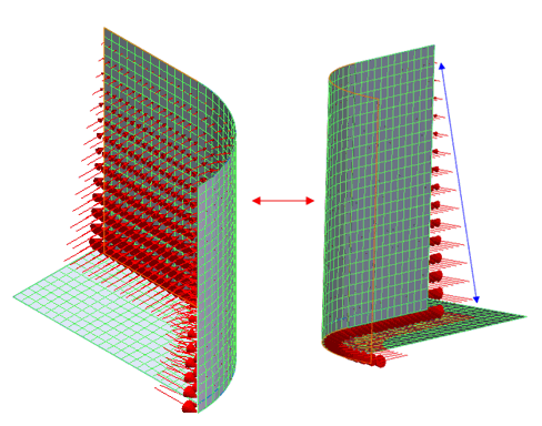
Example 2: Simple 2D Variation on Cylindrical Surfaces
To define a variable load on cylindrical surfaces (ex: bearing load), it is recommended to use the Linear option rather than Linear (Equation Based), as shown in the image below.
-
Example 3: Simple 2D Variation of Hydrostatic Load
To define a hydrostatic variable load, it is recommended to use the Linear (Equation Based) option rather than Linear, as shown in the image below
-
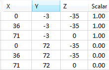
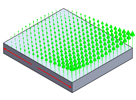
Example 4: Simple 3D Variation on Flat Surfaces
Using the same scalar surface points on a surface creates the following load distribution. The load distribution levels off to 1.0 (the unit value) the further the location from the data points.
-
Linear
-
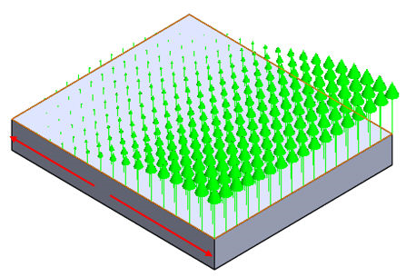
Quadratic
-
Linear