Properties and their Variation Methods

There are several basic properties that are needed to define a fluid. Most of these properties can be made to vary with temperature, pressure, or scalar, in several different ways. The following table lists the properties and the available variation methods.

Property	Variation Methods
Density	Constant, Equation of State, Polynomial, Inverse Polynomial, Arrhenius, Thermodynamic Tables, Piecewise Linear, and Moist Gas Please see note below about specifying density and the gas constant to incorporate real gas effects.
Viscosity (Dynamic viscosity)	Constant, Sutherland, Power Law, Polynomial, Inverse Polynomial, Non-Newtonian Power Law, Hershel-Buckley, Carreau, Arrhenius, Piecewise Linear, and Thermodynamic Tables, First Order Polynomial, Second Order Polynomial
Conductivity	Constant, Sutherland, Power Law, Polynomial, Inverse Polynomial, Arrhenius, Thermodynamic Tables, Piecewise Linear
Specific Heat	Constant, Polynomial, Inverse Polynomial, Arrhenius, Thermodynamic Tables, Piecewise Linear
Compressibility	Cp/Cv (gamma, the ratio of specific heats) -- useful only for compressible gas analyses or Bulk Modulus -- useful only for compressible liquid analyses. See note below.
Emissivity This is useful for radiation analyses. The emissivity specified on a fluid is assigned to contacting walls. Note that the emissivity assigned to a solid overrides the value assigned to a contacting fluid.	Constant Piece-wise Linear variation with temperature. (This is useful for spectral radiation analyses.)
Wall Roughness Useful for simulating variable roughness height for including the effects of friction.	Constant. See note below about the Wall Roughness property.
Phase Use for cavitation simulations.	Specify the vapor pressure or a related material that contains the vapor properties.

To Define Density to Incorporate Real Gas Effects

To simulate real gas effects while still using the Ideal Gas Law, modify the Gas constant on the Density property of the Fluid Material Editor to the consistent with the real gas. For a multi-species gas, calculate the density using:

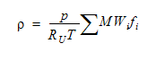
where P is the absolute static pressure, Ru is the Universal Gas Constant, T is the absolute static temperature, MWi is the molecular weight of species i and f i is the mole fraction of species i.

To incorporate this gas into Autodesk® CFD, modify the Gas Constant on the Fluid material editor according to:

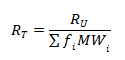
where RT is the value that you would enter on the Autodesk® CFD window for the Gas Constant.

Bulk Modulus

The bulk modulus and the density of a liquid are key to determining the speed of sound through that liquid:

The definition of bulk modulus is:

Given that the speed of sound, a, is defined as:

This works out to be:

Source: White, F. M., “Fluid Mechanics,” McGraw Hill, New York, New York, 1986.

The bulk modulus is used only for compressible liquid (water hammer) analyses. The value of bulk modulus is automatically set for the liquid materials included in the Material Data Base. For user-defined materials, the correct value of bulk modulus is only required if liquid compressibility is to be analyzed. An example of a liquid compressibility, water hammer, is described:

Water is flowing through a straight pipe at 10 in/s. At a certain time, a valve at the end of the pipe is suddenly closed. A pressure pulse will move through the water at the speed of sound through water. This phenomena is called a “water hammer”, and is analyzed with a transient analysis to predict the movement of the pressure wave through the water. Instead of using the Ideal Gas Law and the ratio of specific heats to determine the sound speed, we will use the density and the bulk modulus of the water.

Wall Roughness

Enter a physical dimension (in the units available in the drop menu) of the roughness height. Such heights are typically very small--cast iron pipes, for example, have a typical wall roughness height of 0.0102 inches.

A value of wall roughness height specified on a fluid is automatically applied by the Solver to the wetted walls touching that fluid. A value of wall roughness height specified on a solid is applied to all wetted surfaces (surfaces contacting a fluid) of the part. A non-zero wall roughness height applied to a solid will prevail over a wall roughness applied to a fluid that touches it.

Wall roughness heights are implemented into the turbulence wall model, and do not affect the geometry. The flow must be turbulent for wall roughness heights to take effect. They will be ignored for laminar flows.

Specified wall roughness heights work best when closely adhered to the Turbulent Law of the Wall. This means that the non-dimensional distance (y+) from the wall node to its near-wall node must be between 35 and 350. To automatically vary the mesh wall layer thickness to ensure proper Y+ value, enable Adaptation on the Solve dialog, and check Y+ Adaptation.