Designations adopted:
E - Young's modulus
G - shear modulus
ν - Poisson's ratio
fd - limit of elasticity
Ax - cross section area
Ix - torsional constant
Iy - moment of inertia - bending in XZ plane
Iz - moment of inertia - bending in YZ plane
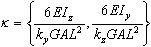
ky, kz - correction coefficients for shear rigidity in Y and Z directions
L - bar length.
-
Preliminary remarks and assumptions
The following assumptions have been adopted for bar (beam) elements:
- Uniform formulation for 2D and 3D (2d & 3D frames, grillages)
- Uniform element allowing for material and/or geometrical non-linearity
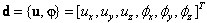
- Standard displacement degrees of freedom at 2 extreme nodes
- Use of the following is allowed:
- Shear deformation included (Timoshenko's model).
- Tapered cross section - only for geometrical non-linearity.
- Winkler's ground.
- There are 2 levels of geometrical non-linearity available: P-Delta (second order theory), and Large displacements which is the most accurate theory possible with large displacements and rotations; this is an incremental approach with a geometry update.
- Assuming small displacements and absence of physical non-linearity for the limit, the results are identical as for standard linear elements.
- In the material non-linearity analysis the layered model and the constitutive stress-strain principle for the uni-axial stress-strain on the point (layer) level are applied.
- Shear and torsion states are treated as linearly elastic and have to be uncoupled from axial forces and bending moments on the cross section level.
- Non-linear releases and hinges may be defined only as DSC elements.
- All types of element loads are allowable (identically as for standard elements). However, it is assumed that nodal forces acting on a structure are determined at the beginning of the process. The changes in the transfer of element loads onto nodes resulting from geometrical or material non-linearity are ignored.
- Apart from the elasto-plastic element, it is also possible to generate elasto-plastic hinges in selected bar cross sections as an extension of the "non-linear hinges" option (see point 5).
-
Geometry, kinematics and strain approximation
Geometry, sign convention for forces, displacements, stresses and strains
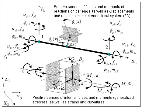
Basic kinematic relationships
In the element local system and in the geometrically linear range, the generalized strains E on the cross section level are as follows (symbol (
 indicates calculation of the differential along the direction of the bar axis):
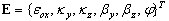
where:
Axial strain in the bar axis:
e0x = u ,x
Curvatures:
K y = fy'x
K z = - f z'x
Average angles (strain):
b y = n 'x - f z'
b y = w 'x - f y
Unit torsion angle:
j = f x'x
Displacement approximation
When there is a possibility to consider shear influence and consistence of results obtained for the linear element, physical shape functions considering shear influence have been implemented.
2D bars:
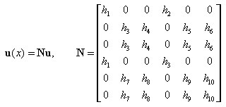
Shape functions and their derivatives are expressed by the formulas:
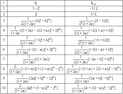
where:
x = x / L
 for planes XY and XZ, respectively.
 Kinematic relationships for the matrix notation (the geometrically linear theory)
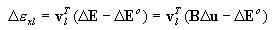
When considering the influence of imposed strains
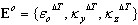
Increment of generalized (sectional) strains:
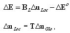
2D:
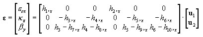
3D:
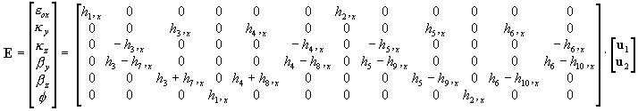
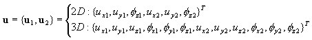
where:
Strains at a point (layer)
Given the generalized strains {ε 0x, k y , k x } of a cross section, the e xl strain or its increment De xl at any point of the cross section l - of the coordinates yl, zl, is calculated as
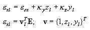
finally, strain increment in the layer:
-
Stresses and internal forces within an element
The constitutive principle on the point level
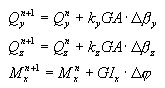
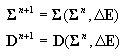
The principle is adopted in the general incremental form, where current stresses σx n+1 are defined as a function of stress for the last equilibrium σx n and current strain increment with imposed (thermal) strains considered,
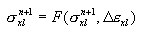
based on the function σ = f(ε) which describes the relationship in the process of active loading and on the specification of the principle of unloading and reloading. In particular, it may be the elasto-plastic principle with linear hardening and the specified principle of unloading, such as (a) elastic, (b) plastic, (c) damage, (d) mixed. For elastic unloading the passive and active process is performed along the same path σ = f(ε). For the remaining ones, it is performed along the straight line determined by the beginning point of a given unloading process {ε UNL, σ UNL } and the unloading module D UNL defined as

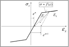
e n is a memorized strain, for which the current active process has started, commenced after exceeding 0 by stresses with the unloading (e 1 = 0) assumed.
For the analysis it is necessary to provide the current stiffness assumed to be a derivative

Calculation of forces and cross section stiffness values.
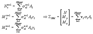
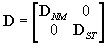
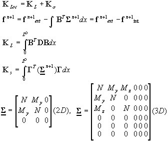
On the cross-section level, the vector of internal forces (stress resultants) is composed of:
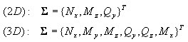
States of shear and torsion ΣST are treated as linearly elastic and not conjugated with the state of axial/bending forces on the cross section level.
Compression/tension states Σ NM are generally treated as conjugate when applying the layered approach. However, as long as the elastic state is guaranteed, i.e. until the current generalized strains fulfil the following elastic state condition:
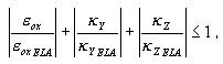
where:

the cross section is treated as elastic and the layered approach is not activated.
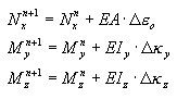
Once violation of the elastic state condition is asserted, stresses induced by axial strains and bending are calculated separately for each layer and on their basis sectional quantities are calculated
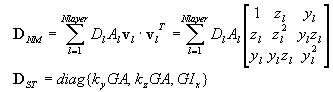
Stiffness on the level of D cross section is calculated as follows:
in the elastic state as:
D = diag {EA, EIy, EIz, KyGA, kzGA, GIx)
After exceeding the elastic state condition as:
where:
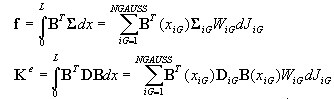
Nodal force vector and element stiffness matrix
They are calculated by means of the standard formulas applying Gauss quadrature (Ngauss=3).
-
Geometrical non-linearity
The following configurations are taken into consideration:
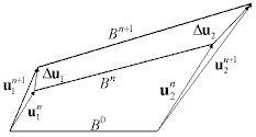
B0 - initial configuration
Bn - reference configuration (the last one for which equilibrium conditions are satisfied)
Bn+1 - current configuration (iterated).
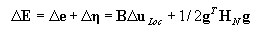
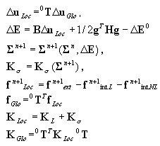
An entry point for the element formulation is the virtual work principle saved in the following form for displacement increments:

where: Δε strain increment while moving Bn to Bn+1, Δe, Δη constitute its parts, correspondingly: linear and non-linear with respect to the displacement increment Δu, whereas τ is a stress referring to the reference configuration and Cijkl is a tensor of tangential elasticity modules.
The Non-linearity option
It corresponds to the non-linear formulation, or the second order theory. Since material non-linearity is possible, the incremental formulation is being introduced (however, without modification of element geometry).
Kinematic relations
Strain increments in the matrix notation:
where:
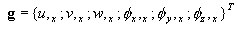
then the displacement increment gradient g = ΓΔu

whereas
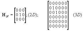
is a selection matrix.
Nodal force vector and element stiffness matrix
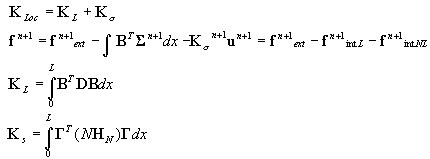
Algorithm on the element level
The element geometry is not modified; the local-global transformation is performed with the use of initial transformation matrix 0 T
Large displacement option
It is a certain variant of bar description allowing for large displacements. The approach of the updated Lagrange description is applied here.
Nodal force vector and element stiffness matrix
-
Elasto-plastic hinges
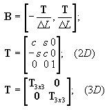
Alternatively, the elasto-plastic work of a structure can be modeled by introducing non-linear hinges at selected bar cross sections. Characteristics of a hinge represented by a 2-node DSC element are defined applying the cross section analysis algorithm described in point 3, assuming that the role of generalized strains E is played by mutual node displacements (with respect to bar local directions) divided by the adopted (fictitious) element length (ΔL) that equals the minimum cross section height. These act as the element volume dV=ΔL. Forces and displacements of newly-generated nodes of the DSC element constitute global degrees of freedom, in other words, they do not undergo condensation.
Algorithm on the element level-
calculation of generalized strains in a cross section

-
calculation of internal forces (stress resultants) and cross section rigidity according to point 3.2
-
calculation of forces (reactions on bar ends) and DSC element rigidity
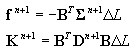
where:
-