Residual stress shrinkage prediction method (MP and DD)

The residual stress shrinkage prediction model has been formulated assuming linear thermo-viscoelastic material behavior. It accounts for the stress developed while the material cools under pressure in the mold. In this method, rather than calculate shrinkage strain we directly calculate a residual stress distribution for each element.

The residual stress distribution provides the stress across the thickness of each element in directions parallel and perpendicular to flow. This stress distribution is then input to the Stress analysis program to obtain the deflected shape of the part. If in addition experimental shrinkage data is available for the material, considerably more accurate prediction of shrinkages and hence part deflections can be obtained than using the residual strain method.

General description of the method

The model has been formulated assuming linear thermo-viscoelastic material behavior. It accounts for the stress developed while the material cools under pressure in the mold. In particular, the model accounts for the thermally induced stress which arises from freezing and subsequent shrinkage of the material as well as the pressure induced stress. The latter stress is caused by the action of the melt pressure on the solidified material forming the frozen layer. Being theoretically based, this model has the advantage that it can be used even if no shrinkage data is available for the material. However, its performance can be improved greatly when shrinkage data is available.

The prediction of shrinkage and warpage is based on the computed thermally and pressure induced residual stress distribution. The computational procedure in the present development is listed below. This is for fiber-filled materials. For unfilled materials the procedure is similar, but there is no need for the mechanical property calculation.

For each time step:

Calculate fluid mechanics:
- Pressure p, Flow rate Q...
- Fiber orientation
Calculate heat transfer:
- Temperature T
- Frozen layer
Calculate thermodynamics:
- f (p, v, T)=0
Update viscosity.
Does the solution converge?
- If NO, repeat from Step 1.
- If YES, go to Step 6.
Calculate micro-mechanics:
- Thermo-mechanical properties:
Calculate thermoviscoelasticity:
- Thermally and pressure induced stresses
If , go to the next time step (repeat from Step 1).

Note: When the Residual Thermal Stress shrinkage model is selected, the Warp analysis uses the asymmetric information produced by the asymmetric Fill+Pack analysis. The asymmetry could be caused by temperature differences between the two sides of the mold or/and by branching geometry. Therefore, even if there is no Cool analysis result, the warpage results could show some asymmetric effects if the part has branching geometry. However, if the Fill+Pack analysis is symmetric, then the Warp analysis will be symmetric and therefore ignore differential cooling.

Application of this method with no shrinkage data

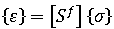
A general form of the anisotropic stress-strain relation for linear thermoviscoelasticity may be written as

where:

and are tensors defining the mechanical and thermal characteristics of the material, respectively.
is a pseudo-time scale which accounts for the temperature dependence of the material and is defined by

where is the time-temperature shift factor characterized by either the WLF equation or the Arrhenius equation depending on the material and the temperature range.

The thermo-viscoelastic model has been found to be extremely sensitive to material data and indeed material data is not readily available for its use. In the absence of experimentally obtained viscoelastic data, we have utilized a viscous-elastic model with two forms:

For non-fiber-filled materials, the model is isotropic whereby the mechanical property tensor is defined by the modulus and Poisson's ratio of the material, as stored in the Autodesk Moldflow materials database, and the thermal expansion coefficients used to define the thermal property tensor are obtained from the pvT data for the material.
For fiber-filled materials, these tensors are defined using anisotropic mechanical and thermal properties for the composite material, which are calculated from the fiber orientation distribution obtained from the Fill+Pack analysis. In this case the model predicts stresses along and transverse to the fiber orientation direction.

The viscous-elastic model is based on the following assumptions:

There is no stress build up in the material until the material is below the transition temperature.
With respect to the local element coordinates in which the x3 direction is normal to the local midplane, the shear stresses = .
The normal stress is constant across the thickness.
As long as < 0 , the material sticks to the mold walls.
A constrained quench condition is prescribed in all the cases as long as the material is in the mold.
Mold elasticity is neglected. (Elasticity of mold cores is taken into account in a core shift analysis.)
The material behaves as an elastic solid after the part is ejected.

This model is available for use with all materials on the Autodesk Moldflow materials database, whether they have undergone shrinkage characterization or not. In the case of fiber-filled materials, the model requires that the option to perform Fiber orientation analysis if fiber material be selected in the Process Settings Wizard-Fill+Pack Settings dialog.

This model is capable of predicting shrinkage trends but can have substantial errors with regard to the absolute values obtained. It is useful for designing to reduce warpage but absolute values are less accurate than when shrinkage data is available. For unfilled materials, the model is isotropic as there is no facility to calculate the effects of molecular orientation or crystallinity in the flow analysis software.

Application of this method when shrinkage data is available

The main factors affecting the accuracy of the prediction from the theoretical model described above are:

Sensitive dependence of shrinkage on transition temperature and pvT data which, using the current measurement methods, cannot represent the behavior under actual injection molding conditions.
No provision for determining molecular orientation and hence for unfilled materials the model does not predict anisotropy.
Lack of provision for crystallinity effects.
Lack of relaxation spectrum data for the viscoelastic calculation.

When a material has been shrinkage characterized by Autodesk Moldflow, the thermo-viscous-elastic model can be improved dramatically by accounting for the measured shrinkage results. This is done by using the theoretical model as one of the independent variables in a hybrid model that is correlated with measured shrinkage data in order to reduce the discrepancy between measured and predicted shrinkage. The resulting model is called a Corrected Residual In-Mold Stress (CRIMS) model.

The idea is illustrated below:

Corrected Residual In-Mold Stress (CRIMS) model

(a) Predicted Isotropic Residual Stress , (b) Error Correction, (c) Corrected anisotropic residual stress and , (d) Measured Shrinkage.

To illustrate the effect of this, consider the following graph.

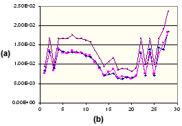
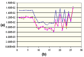
Parallel Shrinkage of Polypropylene

(a) Shrinkage %, (b) Molding Condition Set Number, Measured Parallel, Corrected Parallel, Calculated the critical (isotropic).

This graph shows the experimental shrinkage measured parallel to the flow direction for a polypropylene. Also shown are the theoretically calculated values of parallel shrinkage (using the thermo-viscous-elastic model) and the corrected value of parallel shrinkage. It is clear that the corrected values are in excellent agreement with the measured values. Similar improvement is noted in the perpendicular direction for the same polypropylene as shown below.

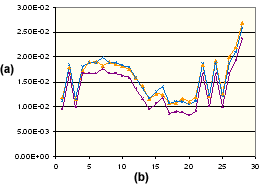
Perpendicular Shrinkage of Polypropylene

(a) Shrinkage %, (b) Molding Condition SetNumber, Measured Perpendicular, Corrected Perpendicular, Calculated the critical (isotropic).

The correction concept also may be applied to fiber filled materials where it also gives excellent results. Below are some results on a PA66 that has 15% by weight of glass fiber reinforcement.

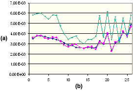
Parallel Shrinkage of PA66 15% GF

(a) Shrinkage %, (b) Molding Condition SetNumber, Measured Parallel, Corrected Parallel, Theoretical Parallel.

Perpendicular Shrinkage of PA66 15% GF

(a) Shrinkage %, (b) Molding Condition SetNumber, Measured Perpendicular, Theoretical Perpendicular, Corrected Perpendicular

Application of this method with single variate analysis

Single variate analysis is a technique provided in the Autodesk Moldflow Warp analysis product to isolate the dominant cause of warpage and allow you to take targeted measures to reduce part warpage. It is discussed in detail in the Single Variate Analysis topics. Here we will consider how the residual stress method is applied in the single variate analysis context.

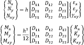
The Fill+Pack analysis of the filling and packing phases outputs the following information which serves as input for the residual stress calculations:

Generalized forces data, i.e., the membrane forces ( ) and bending moments ( ), on each element in the local elemental axis system,
Material orientation angles for each element,
Mechanical properties for each element (the longitudinal Young's modulus, the transverse Young's modulus and the Poisson's ratio).

Single variate analysis is based on the concept that the causes of warpage fall into three categories:

Differential cooling,
Differential shrinkage,
Orientation effects.

This concept is concerned with shrinkage rather than stresses. Therefore, to isolate the cause of warpage in terms of the above three effects when using the residual stress model, we need to calculate generalized strains from the given generalized forces, then decompose the strains into components due to the differential cooling, different shrinkage and orientation effects, and finally convert the modified strains back into corresponding generalized forces. Separate stress analyses are then performed to obtain warpage results for each effect. The relevant equations for the calculations are summarized below.

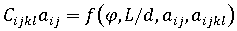
Hooke's law for a transversely isotropic material (the mechanical properties are isotropic in all planes perpendicular to the fiber axis , that is axis 1) can be expressed as:

where

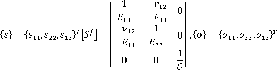
, and the compliance matrix is given by

Alternatively, Hooke's law can be written in terms of a stiffness matrix as follows

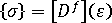
with

Given the material orientation angle , we transform the compliance matrix and the stiffness matrix from the oriented system to the local elemental system.

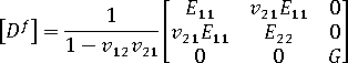
The generalized strains are given by

where and are the strain and the curvature vectors respectively.

The following equations convert the strains and the curvatures back to the membrane forces and bending moments:

To isolate the effects of warpage, we replace and by the decomposed components, then recalculate the membrane forces and bending moments and use the new values in the structural analysis.