Pipe calculation information

For modelling purposes, InfoWorks WS Pro sub-divides links.

A pipe is represented in the model by:

• two terminal nodes ("i" and "j")
• length, L (m)
• internal diameter, D (mm)
• friction coefficient,λ
• sum of local head-loss coefficients, ζ

The friction coefficient is used to calculate the headloss along a pipe. In the InfoWorks simulation engine, headloss is always calculated using the Darcy Weisbach formula.

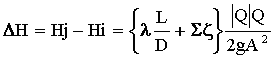
(1) where: (2) and: Q > 0 if Hj > Hi Q is negative if Hj < Hi

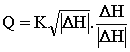
For the "node-oriented" method this equation is often written as:

(3) where: (4)

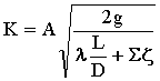
K is a measure of capacity of the pipe. K depends upon the value of Reynolds number Re .

(5) where: is the coefficient of kinematic viscosity

You can enter a friction coefficient in the format for one of three friction formulae:

• Darcy Weisbach
• Hazen Williams
• Colebrook White

InfoWorks then converts the friction coefficient using methods described below.

Darcy Weisbach

The parameter λ entered by the user is used directly. λis non-dimensional.

Hazen Williams

The Hazen Williams friction formula:

(6) where: m = 4.8704 n = 1.852 C is the friction coefficient

InfoWorks uses the following relationship to convert C to the Darcy Weisbach friction coefficient λ:

(7)

The equivalent Darcy-Weisbach factor is dependent on the Reynolds number for flow in each pipe and is re-evaluated at each iteration of the simulation.

Note: If the Use dynamic friction factors option is not selected in the Simulation Options dialog, InfoWorks converts the Hazen Williams coefficient C to a Darcy-Weisbach friction coefficient only once for each pipe, assuming a flow speed of 1 m/s.

Colebrook White

The user may decide to specify Colebrook White internal roughness k.

The equivalent Darcy-Weisbach friction factor, λ, is modelled on the Moody diagram, is dependent on the Reynolds number (Re) for flow in each pipe and is re-evaluated at each iteration of the simulation.

Note: If the Use dynamic friction factors option is not selected in the Simulation Options dialog, InfoWorks converts the Hazen Williams coefficient C to a Darcy-Weisbach friction coefficient only once for each pipe, assuming a flow speed of 1 m/s.

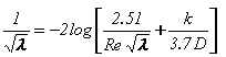
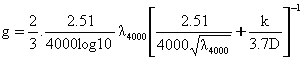
For Re >= 4000, InfoWorks solves the Colebrook-White equation iteratively to convert the specified internal roughness k to the Darcy-Weisbach friction coefficient to an accuracy of 0.1%:

(8)

For Re < 4000 there are two methods for modelling the Moody diagram in the critical zone between laminar flow and the transition / turbulent zone.

• Cubic spline interpolation
• Modified CW-Moody (constant value)

The Modified CW-Moody method is the most stable numerically and for this reason is set as the default method in the Simulation Options dialog. Although this option may over-estimate the friction factor, this generally only occurs for low pipe flows and any hydraulic effects are not likely to be significant.

Cubic Spline Interpolation

For 2000 < Re < 4000, a cubic polynomial interpolation using standard cubic spline methods to match the laminar friction factor at Re = 2000, the Colebrook-White derived value at Re = 4000(λ ₄₀₀₀) and their respective gradients:

(9) where:

For Re <= 2000, the friction factor is calculated from the Hagen-Poiseuille formula for laminar flow:

(10)

Modified CW-Moody (constant value):

For 2000 < Re < 4000, a constant value is imposed equal to the friction factor calculated from the Colebrook-White equation at a Reynolds number of 4000:

λ = λ 4000 (11)

For Re <= 2000, the friction factor is the maximum of the Hagen-Poiseuille formula for laminar flow and the constant value above with a maximum cut-off value of 8 for Re<= 8.

(12)