Various transition curves are used in civil engineering to gradually introduce curvature and superelevation between both straights and circular curves as well as between two circular curves with different curvature.
In its relationship to other tangents and curves, each spiral is either an incurve or an outcurve.
The two most commonly used parameters by engineers in designing and setting out a spiral are L (spiral length) and R. The R parameter refers to the radius of curvature at one end of the spiral. R1 and R2 may be used to differentiate between the radius at the start and end of the spiral.
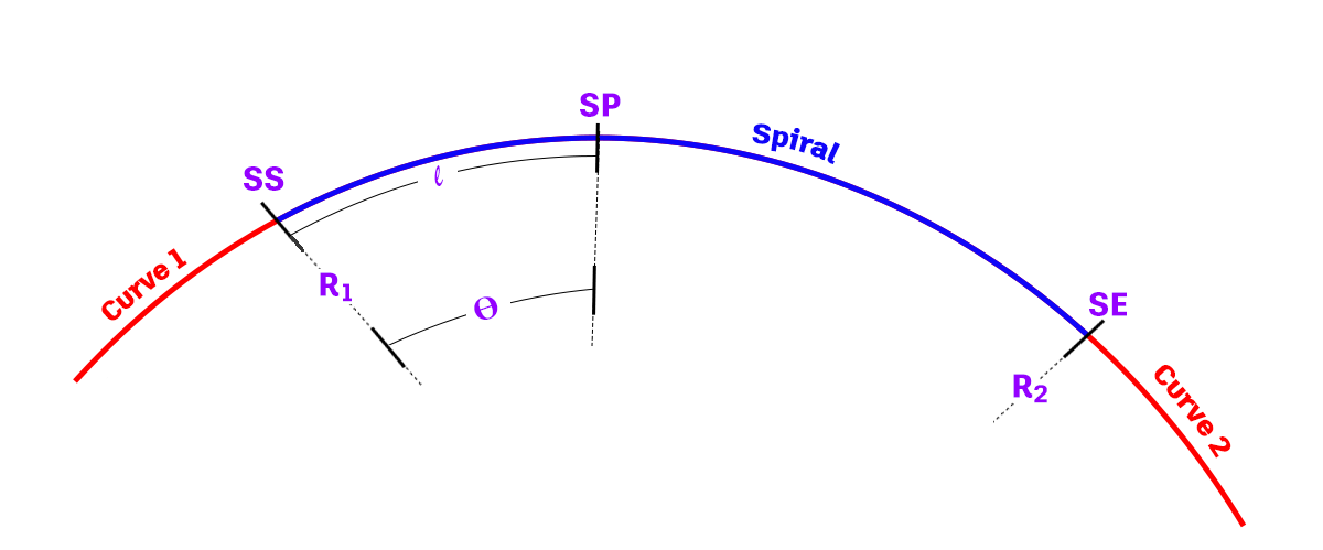
The following illustration shows the various parameters of a transition:
| Spiral Parameter | Description |
| R1 | The radius of curve 1. |
| R2 | The radius of curve 2. |
| SS | The spiral start position. |
| SE | the spiral end position. |
| SP | The spiral point at arc length l. |
| Θ | The central angle at the spiral point at arc length l. |
| l | The arc length from the spiral start position along the spiral. |
| L | Total arc length of the spiral between the spiral start and end positions. |
Compound Transition
Compound transitions provide a transition between two circular curves with different radii. There are two spiral types: simple and compound. A compound spiral consists of a curve composed of two simple spirals. It contains two spans, each of which is a simple spiral, joining tangent continuously with its adjacent spiral. This allows for continuity of the curvature function and provides a way to introduce a smooth transition in superelevation.
Clothoid Spiral
While Autodesk Civil 3D supports several spiral types, the clothoid spiral is the most commonly used spiral type. The clothoid spiral is used world-wide in both highway and railway track design.
First investigated by the Swiss mathematician Leonard Euler, the curvature function of the clothoid is a linear function chosen such that the curvature is zero (0) as a function of length where the transition meets the straight. The curvature then increases linearly until it is equal to the adjacent curve at the point where the transition and curve meet.
Unlike the simple curve, it also maintains continuity of the local curvature, which is increasingly important for vehicles at higher speeds.
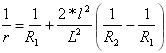
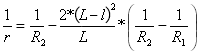
Formula
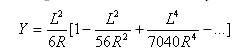
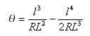
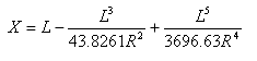
Clothoid spirals can be expressed in the following formulas: ![]()
- Θ= The central angle at the spiral point at arc length l.
- l = The arc length along the curve.
Flatness of transition: ![]()
Total angle subtended by transition: ![]()
Straight distance at transition-curve point from straight-transition point is:
Straight offset distance at transition-curve point from straight-transition point is:
Bloss Transition
Instead of using the clothoid, the Bloss spiral can be used as a transition. This transition has an advantage over the clothoid in that the shift P is smaller and therefore there is a longer transition, with a larger transition extension (K). This factor is important in rail design.
Formula
Other key expressions:
Straight distance at transition-curve point from straight-transition point is:
Straight offset distance at transition-curve point from straight-transition point is:
Sinusoidal Curves
These curves represent a consistent course of curvature and are applicable to transition from 0 through 90 degrees of straight deflections. However, sinusoidal curves are not widely used because they are steeper than a true transition and are therefore difficult to tabulate and stake out.
Formula
- Θ= The central angle at the spiral point at arc length i.
- l = The arc length along the curve.
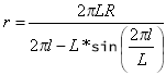
Where r is the radius of curvature at any given point.
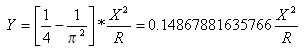
Sine Half-Wavelength Diminishing Straight Curve
This form of equation is commonly used in Japan for railway design. This curve is useful in situations where you need an efficient transition in the change of curvature for low deflection angles (in regard to vehicle dynamics.)
Formula
Sine Half-Wavelength Diminishing Straight curves can be expressed as:
Where ![]() and x is the distance from the start to any point on the curve and is measured along the (extended) initial tangent, X is the total X at the end of the transition curve.
and x is the distance from the start to any point on the curve and is measured along the (extended) initial tangent, X is the total X at the end of the transition curve.
Other key expressions:
Straight distance at transition-curve point from straight-transition point is:
Straight offset distance at transition-curve point from straight-transition point is:
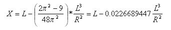
Cubic Parabolas
Cubic parabolas converge less rapidly than cubic transitions, which makes their use popular in railway and highway design.
Formula
Minimum Radius of Cubic Parabola
Where: Θ= The central angle at the spiral point at arc length  .
.
See the diagram above for reference.
A cubic parabola attains minimum r at:
So ![]()
A cubic parabola radius decreases from infinity to ![]() at 24 degrees, 5 minutes, 41 seconds and from then onwards starts to increase again. This makes cubic parabolas useless for deflections greater than 24 degrees.
at 24 degrees, 5 minutes, 41 seconds and from then onwards starts to increase again. This makes cubic parabolas useless for deflections greater than 24 degrees.
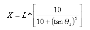
Cubic (JP)
This transition was developed for requirements in Japan. Some approximations of the clothoid have been developed to use in situations to accommodate a small deflection angle or a large radius. One of these approximations, used for design in Japan, is Cubic (JP).
Formula
Cubic (JP) can be expressed as:
Where X = Straight distance at transition-curve point from straight-transition point
This formula can also be expressed as:

Where ![]() is the central angle of the spiral (illustrated as i1 and i2 in the illustration)
is the central angle of the spiral (illustrated as i1 and i2 in the illustration)
Other key expressions:
Straight distance at transition-curve point from straight-transition point is:
Straight offset distance at transition-curve point from straight-transition point is:
NSW Cubic Parabola
This is a type of modified cubic parabola to meet the requirements of New South Wales (Australia) standards.
Formula
The NSW cubic parabola can be expressed as:
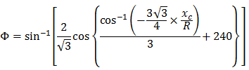


- Φ = angle between final radial line at R and perpendicular line to the initial straight
- R = radius of curve
- Xc = total X of the given spiral
- Yc = total Y of the given spiral
Bi-Quadratic (Schramm) Transitions
Bi-quadratic (Schramm) transitions have low values of vertical acceleration. They contain two second-degree parabolas whose radii vary as a function of curve length (l).
Simple Curve Formula
Curvature of the first parabola:
![]() for
for ![]()
Curvature of the second parabola:
![]() for
for ![]()
This curve is specified by the user-defined length (L) of the transition curve.
Compound Curve Formulas
Curvature of the first parabola:
 for
for ![]()
Curvature of the second parabola:
 for
for ![]()