Subjects Covered

• Wind Load
• Differential settlement
• Lack of fit loading
• Dead loading
• Bending Moment, shear and Axial force diagrams

Outline

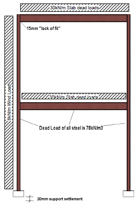
The portal frame model, created in example 6.2, is to be loaded with the following characteristic loads:

1. Dead load of the steel members based upon a weight density of 78kN/m3
2. Dead Load of precast concrete floor panels resulting in a UDL on the beams of 30kN/m
3. A horizontal wind load of 8kN/m acting as a UDL on the left hand columns
4. A support settlement of 20mm applied just to the left hand support

5. A “Lack of fit” loading due to the top beam being 15mm short during erection

   

Create a ULS:STR combination for persistent situations of these loads using load factors of 1.5 for the wind load and 1.35 for all other loads. There is only one variable load (that will have a ψ0 value of 1.0).

Produce a combined bending moment/shear force diagram for the two beams, with max values annotated, and an axial force diagram for the two columns – both for the combined load case.

Procedure

1. Start the program and use the main menu item File | Open... to open the file created in example 6.2 called “EU Example 6_2.sst”.
2. Click on the menu File | Titles... and change the Project Title to “Portal Frame Loading”, the sub title to “Example 7.2”, the Job Number to “7.2” and enter your initials in the Calculated by: field.
3. Close the Titles form using the ✓ OK button.

4. Click on the Structure Loads button at the bottom of the Navigation window to enable adding basic loads into the navigation tree.

   Dead Loads

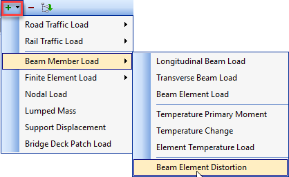
5. Click on the + toolbar button at the top of the navigation window and select Beam Member Load | Beam Element Load from the list of options.

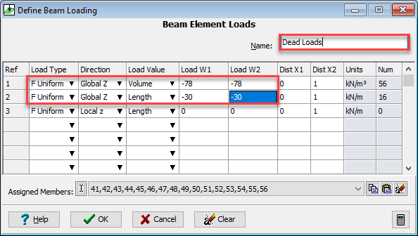
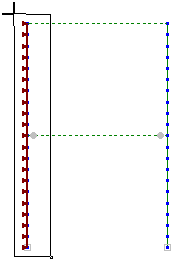
6. We can enter the steel dead load into the first row of the Define Beam Loading form by setting Load Type to be “F Uniform”, Direction to “Global Z”, Load Value to be “Volume” and Load W1 to be “-78” (it is negative because it is acting vertically downward). W2 automatically assumes the same value as it is a uniform load.
7. Click on the small “down arrow” next to the filter button in the graphics toolbar and select “Beam Only” from the list of filters (these filters were set up in example 6.2). Window round the whole structure.

8. Repeat 7 but with the filter “Columns Only”. There should be 56 members now loaded as seen in the last column of the table.

   

   

9. The second line in the table can now be used to define the slab dead loads which will be “F Uniform”, “Global Z”, “Length” and “-30”.

10. This should be applied to just the beams using the “Beam Only” filter.
11. Note the third row in the table is just a prompt and has no members assigned so is ignored. This can be checked in the data reports if necessary.

12. Change the Name: to “Dead Loads” and close the Define Beam Loading form with the ✓ OK button.

    Wind Loads

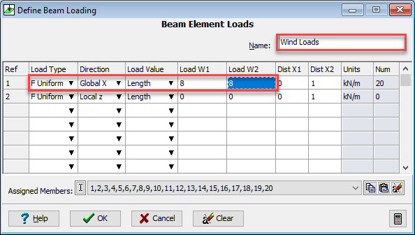
13. The wind load will also be created in a similar way using the + button. Select Beam Member Loads | Beam Element Load. The parameters for this will be: “F Uniform”, “Global X”, “Length” and “8”. It should be applied to just the left hand column by using the “Columns Only” filter but only windowing around the left half of the structure.

    

    

14. Change the Name to “Wind Loads” before closing the Define Beam Loading form with the ✓ OK button.

    Support settlement Load

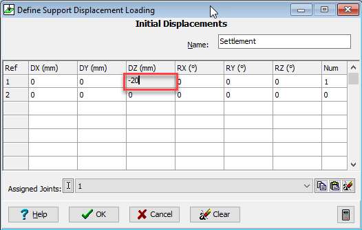
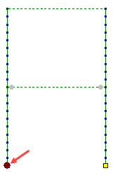
15. Click on the + button at the top of the navigation window and select Support Displacement from the list.

16. Enter “-20” in the DZ(mm) column of the first row and then click on the left supported node in the graphics window.

    

    

17. The default Name of “Settlement” is suitable so close the Define Support Displacement Loading form with the ✓ OK button.

    Lack of Fit Load

18. Click on the button at the top of the navigation window and select Beam Member Load | Beam Element Distortion from the list.

    

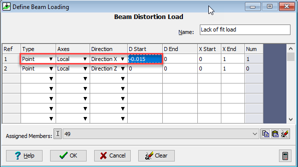
19. The lack of fit can be applied as a point distortion of -15mm at any point along the top beam. Enter “-0.015” in the D Start column of the first row and then set Type to “Point”, Axes to “Local”, Direction to “Direction X”.

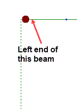
20. Apply this to the structure by setting the filter to “Beam only” and then clicking on left end of the top beam.

    

    

21. Set the Name to “Lack of fit load” and then close the Beam Distortion Load (Define Beam Loading) form with the ✓ OK button.

    Compilation

22. To form a combination of these loads we create a Compilation. Click on the Structure Compilations button at the bottom of the navigation window and then click on the + button at the top. Select Other from the list.

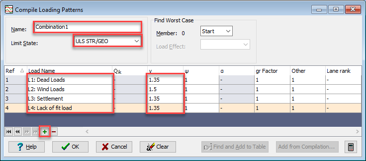
23. In the Compile Loading Patterns form click 4 times on the ”+” button near the bottom of the form add 4 rows to the table. Set the Limit State: to “ULS STR/GEO” and change the Name: to “Combination1”. In the first row of the Load Name field, click and select the “L1: Dead Loads” and set  to 1.35

24. Select each of the remaining loads into separate rows of the table and apply the appropriate factors.

    

25. Close the Compile Loading Patterns form with the ✓ OK button.

    Solution

26. Click on the main menu item Calculate | Analyse Structure... to perform the analysis which will display a form showing the progress of analysing the four load cases. Before closing this form display the analysis log file by clicking on the button.

27. In the text file that is displayed check that the total loads applied in load case L1 are equal and opposite to the support reactions for the same load case. (This applies to direct actions and not moments).

28. Close both the log file and the Analysis form.

    Results

29. Click on the menu item File | Results to open up the results viewer. This can be displayed as full screen if required using the window controls.

30. Use the menu item View | Set Default Layout | Tabbed Layout to set the view to a tabbed view with the Graphics on one tab and the table on another (this will not need doing if it is already a tabbed view). Click on the Graphic tab at the bottom.
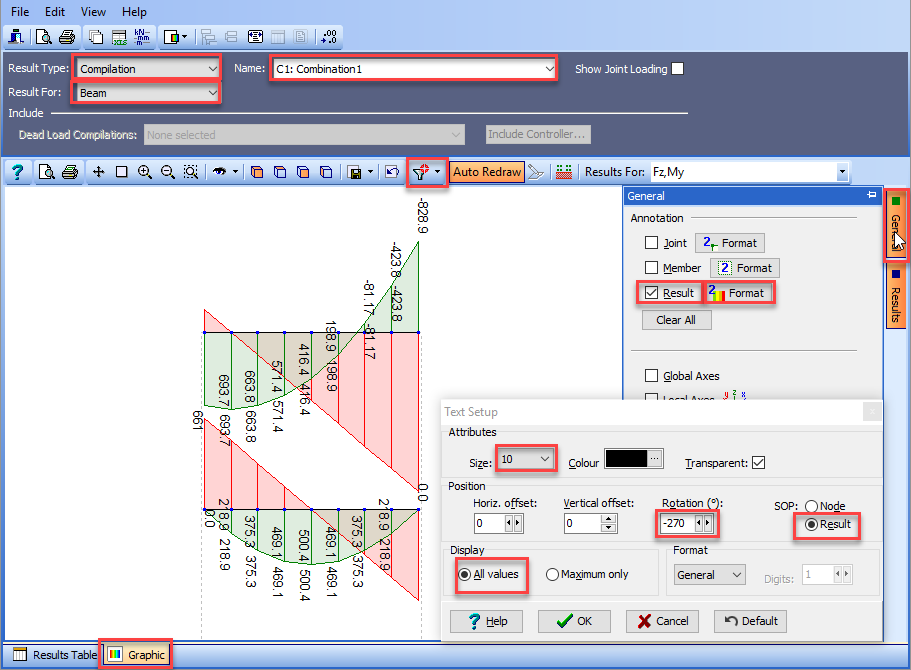
31. In the blue control area Set Results Type to “Compilation”, Name: to “C1: Combination 1”, Results For: to “Beam”.
32. Use the filter dropdown button to select “Beam Only”.
33. Click twice in the Results For field in the light blue graphics toolbar and in the dropdown tick both “FZ” and “MY”.
34. To produce annotations of the values click on the orange General button on the right side of the graphics screen, tick Result and then click the “Format” button next to it.
35. Set the values to the values shown in the following graphic before closing the Text Setup form using the ✓ OK button.

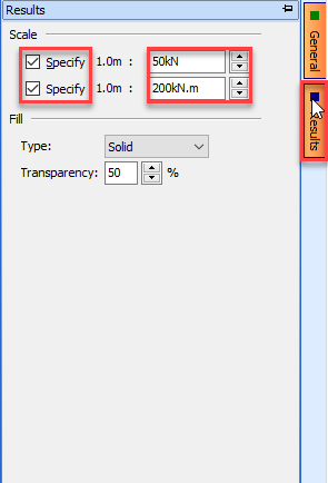
36. To enhance the scale of the plot click on the orange Results button on the right side of the graphics screen and tick both scale boxes setting the scale for shear as 1:50 and that for bending 1:200. (You may want to check that Auto Redraw is switched on. The “Auto Redraw” button is located on the light blue graphics toolbar).

    

    

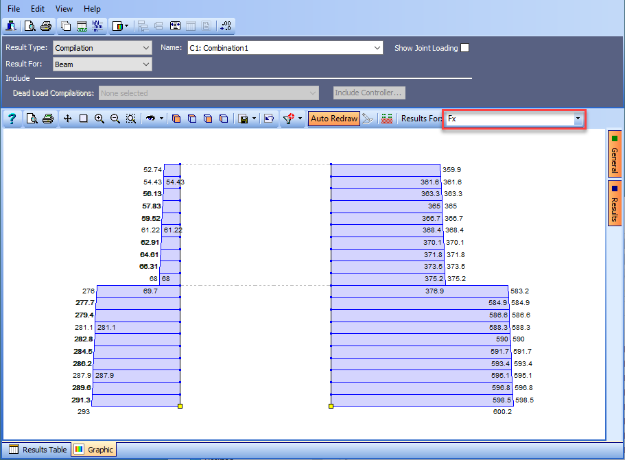
37. A plot of the axial loads in the columns can be obtained in a similar way except the filter would be set to “Columns Only” and the Results For tick box set to “FX” only. For this plot it is best to rotate the results text back to 0.0 using the Text Setup form.

    

38. Close the Results Viewer using the File | Close Tabular Results menu item.

39. Save the file using File | Save as... with a name of “My EU Example 7_2.sst”.
40. Close the program.

Summary

This example explores some of the “not so common” load types applied to portal frames and creating a combination of them. The use of filtering is encouraged to produce graphical and tabular results for just specific parts of the structure and here, excluding parts, such as stiff dummy members, where results are not relevant.

Sometimes the default scale of results plots is not large (or small) enough to show the results adequately. This example shows how user defined scales can visually improve the quality of graphical results.

In results plots that consist of more than one component, (eg. moment and shear) where results values are displayed, then only one component can be annotated at a time. The component that is shown is the first one selected when making the selection in the dropdown list. To change the annotation to another component it is simply a matter of re-selecting the components in a different order.