Subjects Covered

• Beam Loads
• EU Rail Loads
• Compilation
• Envelopes
• Bending Moments
• Graphical Results

Outline

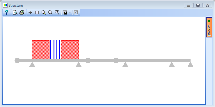
It is required to analyse a five span line beam model as shown below and as defined in example 6.1.

The line beam represents half of a two beam, single track, railway viaduct.

It is required to determine the maximum design sagging moment in spans 2 and 4 for the ULS/STR combination for persistent design cases.

Details of the characteristic loading are as follows:

• Dead load of the beam is 25kN/m³ (γG = 1.35)
• Ballast 0.3m deep x 1.3 (Table NA1 of NA to EN1991-1-1 sub clause 5.2.3(2)). Density 20kN/m³ (γG = 1.35)
• Track and sleepers 5kN/m (2.5 on each beam) (γG = 1.35)
• Live load model 71 assuming a dynamic amplification factor of 1.23 (γQ = 1.45)

Five live load cases should be created for each span, one with the concentrated load at the centre of the span and others with the concentrated load 1m & 2m either side of this. These can then be enveloped.

Procedure

1. Start the program and then use menu item File | Open... to open the data file “EU Example 6_1.sst” which was created in example 6.1.

2. From the main menu select File | Titles to Change the sub title of the example to “Example 7.1”. Set the Job Number to “7.1” and put your initials in the Calculations by: field before closing the form in the normal way.

   Basic Loads

   To calculate the dead load of the beam it is necessary to determine its cross section area so that we can apply the load as a beam load in terms of load per unit length.

3. To do this open up the Data Reports form using the File | Data Reports... menu item. Tick the Structure | Property Data tick box and click on the View button. This will open the Results Viewer which should show the cross section area of the beam as 700000mm². This means the UDL for dead load will be 25 x 0.7 = 17.5kN/m.

4. Click on EXIT to close this window and then on the ✓ Done button to close the Data Reports form.
5. Change the navigation window on the left hand side of the screen to Structure Loads.
6. Click on the toolbar + button and select Rail Traffic Load | Load Model 71.

7. In the Define Rail Traffic Load form change the Ends Defined By: to “span” and Span No: to “2”. Then set Dynamic Factor, Ф: to “1.23”. The intensity of the UDL and concentrated load should be divided by 2 to reflect that only half the load will be applied to one beam. Hence, enter “40kN/m” in the UDL field and “125kN” in the Concentrated Load field (Click OK on the warning messages). Change the Concentrated Load Chainage to “20.5m”.

   

   

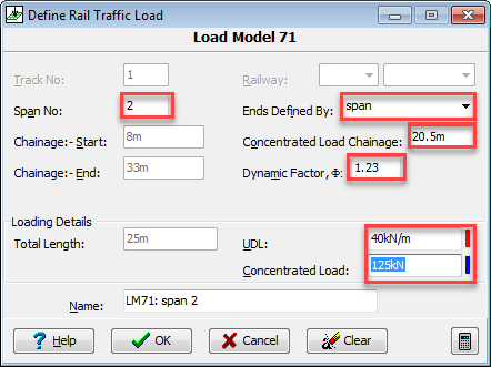
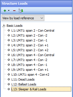
8. Change the Name: to “LM71 Span 2 – Con central” before closing the form with the ✓ OK button.

9. In the Navigation window right mouse click on the “L1” load in the list and select Copy from the context menu. This adds a second load case, L2, and opens the Define Rail Traffic Loading data form. Move the concentrated load 2m to the left by changing the Concentrated Load Chainage: from “20.5” to “18.5”. Change the Name: to “LM71 Span 2 – Con -2” before closing the form with the ✓ OK button.
10. Repeat this for “Con -1”, “Con +1” and “Con +2” changing the concentrated load position and name accordingly.
11. Repeat 6, 7 and 8 for span 4 (Specify Span No. 6 in the data form as this is the virtual span number due to the drop in span) giving 10 live loads in total. (You may have to re-select Ends Defined By: Span to ensure that the loads are correctly defined). (The concentrated load chainage will be “70.5m” for the central case).
12. Click on the + button at the top of the navigation window and select Beam Member Load | Longitudinal Beam Load from the selection list.

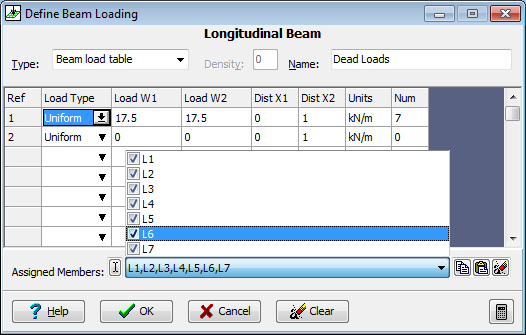
13. In the first row of the Longitudinal Beam Loading form set the Load Type to be “Uniform”, Load W1 to be “17.5” (Load W2 is automatically set as it is uniform) and the Name: to “Dead Loads”. To apply this load to the complete beam, box round the whole structure in the graphics window or tick all members in the drop down list at the end of the Assigned Members: field. Close the form with the ✓ OK button.

    

14. Copy the Dead load in the same manner as for the live loads and change the Load W1 value to “11.7kN/m” and the Name: to “Ballast Loads”.

15. Repeat this again but change the Load W1 value to “2.5” and the name to “Sleeper & Rail Loads”.

    There are now a total of 13 load cases.

    

    Compilations

16. Change the Navigation window to Structure Compilations by clicking the appropriate button at the bottom of the navigation window.

17. Click on the + button to add a Dead Loads at Stage 1 compilation. Click on the “+” button near the bottom of the form to add a row to the table. In the Load Name field use the drop down list to select the beam dead load case. Select “ULS STR/GEO” in the Limit State: drop down and confirm a change of the factors. Ensure that the gamma value is 1.35. Change the Name: to “DL ULS”. Close the form with the ✓ OK button.

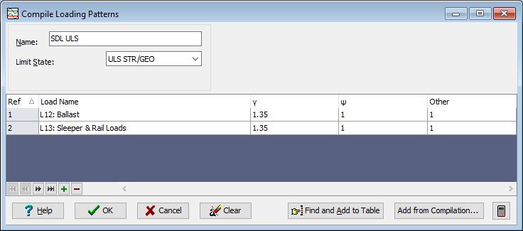
18. Click on the + button to add a Superimposed Dead Loads compilation. Click on the “+” button near the bottom of the form twice to add 2 rows to the table. Select “ULS STR/GEO” in the Limit State: drop down. In the first row of the compilation table select the ballast load case and set the gamma factor to 1.35. In the second row select the sleeper & rail load case and set the gamma factor to 1.35. Set the Name: to “SDL ULS”. Close the form with the ✓ OK button.

    

19. Click on the + button to add a Rail Traffic Groups | GR11 compilation. Click on the “+” button near the bottom of the form to add a row to the table. In the Limit State dropdown select “ULS STR/GEO”. In the Load Name field use the drop down list to select the first live load case. Note that the default Gamma is correct at 1.45. Change the Name: to “Bending Span 2 Con Cen ULS” and close the form with the ✓ OK button.

20. Copy this compilation in the same way as before but change the load case to the second load and change the name accordingly.

21. Create a separate compilation for each live load case in the same way, giving a total of 12 compilations.

    Envelopes

22. To determine the max bending moment in each of spans 2 and 4 we create an envelope. This is done using the main menu item Calculate | Envelopes... to open up the Define Envelopes form.

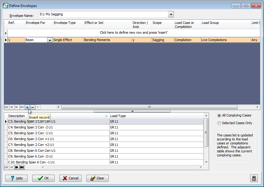
23. 23. Click the mouse where it says “Click Here....” and set Envelope For to “Beam”, and accept all other entries as the default values except the Load Group which should be set to “Live Compilations”. Click on the small “+” button at the bottom of the top part of the table to add this data to the table and because All Complying Cases is selected all live load cases are entered into the envelope automatically. Click on the ✓ OK button to close the Define Envelopes form.

    

24. The load cases can now be solved using the main menu *Item Calculate |Analyse Structure, which carries out the solution and stores results ready for viewing.

    Results

25. The maximum sagging moments can then be obtained by looking at the results of the envelope in the results viewer. This is opened using the main menu item File | Results...

    

26. Set the Results Type: to “Envelope”, the Results For: to “Beam” and the Name to “E1: My Sagging”.

27. If the graphics and tabular results are not shown on the same screen then ensure that the Graphics is enabled using the menu item View | Set Default Layout | Graphic Above Table.
28. To add the effect of dead load and superimposed dead load to the enveloped results then use the drop down list in the Include Dead Load Compilations: field to include both Dead &SDL compilations. (This is located near the top left hand corner of the graphics window).
29. To determine the maximum value then annotate the graphics using the orange “General” button at the right of the graphics screen and tick the Result tick box. If all results are shown then the “Format” button can be used to select maximums only.

    Filtering

30. The overall maximum is in span 2 but if we require to determine the maximum in span 4, the simplest thing to do is to filter the results for span 4 only. This is done by clicking on the graphics filter button .

    

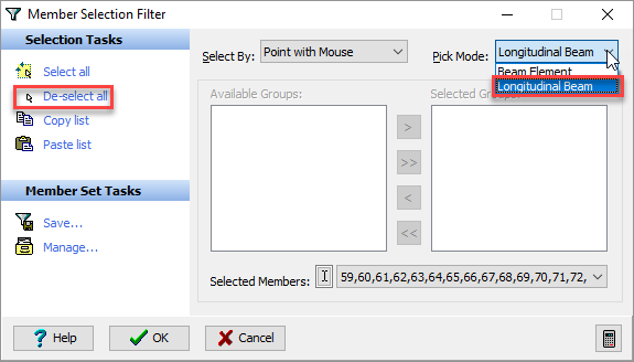
31. First of all De-select all from the Selection Tasks and set the Pick Mode to “Longitudinal Beam”. Then click anywhere on the forth span in the graphics window before closing the Member Selection Filter form with the ✓ OK button. The maximum sagging moment in span 4 is then shown on the graphics.

32. Annotate the member numbers using the General button in the graphics window and also tick “Filtered Members Only”.

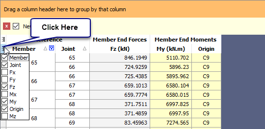
33. Remove columns in the table that have zero values and have no meaning for a line beam analysis by unticking the selection that appears when clicking on the first column of the headings row - as shown below:

    

34. To see how the graphics and table would be printed out, use the File | Print Preview main menu item to display the print preview. When the print preview window is open, a pdf of the graphic window can be generated by clicking on the icon at the top of the print preview window. Close the print preview using the Close button at the end of the toolbar.

35. Close the results viewer using the File | Close Tabular Results main menu item.
36. Save the data file, using File | Save as... with a name of “My EU Example 7_1.sst”.
37. Close the program.

Summary

This example provides a basic introduction to the Analysis modules of Autodesk® Structural Bridge Design and demonstrates the basic principles for assigning properties, defining Eurocode railway loads compilations and envelopes and viewing the results.