10.1 Two Span Prestress Beam Deck

Subjects Covered

Prestressed Precast Beam Structures

Outline

This two span bridge deck is constructed of Y beams (6 in each span with the outer beams being YE beams) acting compositely with a 200mm thick concrete slab.

Two Span Bridge Deck

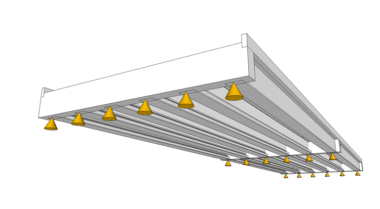
600mm wide diaphragms are cast to the bottom of the beams along the three lines of support and bearings are placed under the ends of the beams. There is a small 300mm deep upstand at the edge of the slab.

Two Span Bridge Deck

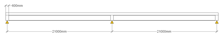
Both spans are 21m from support centre lines which are slightly skewed as shown below.

The slab, diaphragm and upstand are created with grade C32/40 concrete and the prestress beam with grade C50/60 concrete.

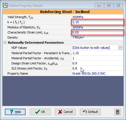
Reinforcement is grade B500B with a ductility factor k of 1.15 and an ultimate strain of 0.05. 25mm diameter bars are placed longitudinally at 200mm centres in the top of the slab with 50mm cover. These bars extend 6m into the slab either side of the central support.

The prestressed tendons have a 0.1% proof strength of 1600MPa.

The structure is modelled using a skewed grillage with vertical offsets so that the centroids of each component are at the correct height.

The construction sequence is firstly to place the beams onto supports so that they carry their own weight. The insitu slab (excluding the edge upstand) is then cast for the first 18m of each span, measured from the free ends, leaving a 6m infill over the central row of supports (the end diaphragms are cast as part of stage 1A). The next stage is to cast the 6m infill slab with the central diaphragm, which, when hardened will make the beams continuous over the central supports. Lastly the upstand is cast.

Two Span Bridge Deck

The carriageway is 18m wide with a 1.5m footway on either side.

It is required to design an adequate prestress strand layout with appropriate debond locations to satisfy all execution and persistent design situations for one of the central inner beams. ULS:STR moments and shears should be checked against section resistance, providing shear reinforcement where required. Section stresses under SLS Characteristic combinations of actions should be checked against material limits for all execution stages as well as persistent design situations for normal use.

The actions to consider on the structure are:

Concrete dead loads assuming 25kN/m³.
Surfacing loads of 2kN/m² over the carriageway and 3kN/m² over the footways.
Crash barrier dead loads of 1.3kN/m along the upstands.
Non linear differential temperature considering a surfacing thickness of 75mm.
Differential shrinkage assuming that shrinkage drying starts after 2 days and that ambient relative humidity is 80%. Both ambient and curing temperatures are 20 degrees C.
Traffic actions from Gr1a and Gr5 combinations with a special vehicle of SV80.

All partial factors, combination factors etc should conform to the values in the UK national annex.

Procedure

The general procedure is as follows:

Create a new project for a line girder and add tiles etc
Define the materials needed
Define 4 prestressed design beams, two edges two inner
Define a two span line beam representing an inner line of beams and assign properties from the design beams
Analyse (automated) for construction, diff temperature and diff shrinkage
Transfer the results for the two spans into the design beam load tables
Save the beam data into beam files by linking the design beams and save the project file
Change the structure type to a refined analysis
Define a grillage structure and any additional design sections required
Define basic loads and compilations for superimposed dead loads
Define traffic load patterns for bending and shear using Influence surfaces and load optimisation procedures.
Change one of the linked beam to an embedded beam an transfer load effects back to it.
Inspect the results and carry out some design checks
Re-link the design beam to update the beam file and save the project file to a new file

Set up and Materials

Start the program and then create a new project using the menu File | New | Create from Template... and select “EU Project”.
Set the correct analysis type using the main menu Data | Structure Type | Line Beam.
From the main menu select File | Titles and set Project Title to “2 Span Prestressed Line Beam” with a sub-title of “Example 10.1” and a Job Number “10.1”.
Add your initials in the Calculations by: field and click ✓ OK to close the form.
In the Materials navigation window, select the C40/50 concrete material to open the Property Details form, and change the cube strength to 60MPa, thus creating a C50/60 grade concrete.
Click ✓ OK to close the form.
Next, click on the Reinforcing Steel material and set the value of k to “1.15” and the Characteristic Strain Limit to “0.05”.
Click ✓ OK to close the form.
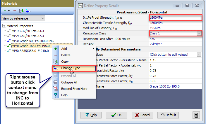
Finally, click on the Prestressing Steel material and then right mouse button click to Change Type to “Prestressing steel – Horizontal”.
Ensure that the 0.1% Proof Strength is set to “1600MPa” and the relaxation class is set to “Class 1” before closing the form with ✓ OK.

Beam Definition

In theory only three different design beams (one internal one north edge and one south edge) are require as the spans and carriageway are completely symmetrical. This is only true if the beam directions can be reversed, which is ok for a refined analysis but unfortunately not for a line beam analysis.

So, four beams are required, one edge and one inner for each span (The north edge in span 1 can also be used for the south edge of span 2 and vice versa). Initially we will create the inner beam for span 1.
In the Design Beam navigation window click on the toolbar button to select New Pre-tensioned Prestressed beam from the available list.
The Beam length is “21m” and Location is “Interior beam”. Cross section is “varying” and No. of different sections is “2”.
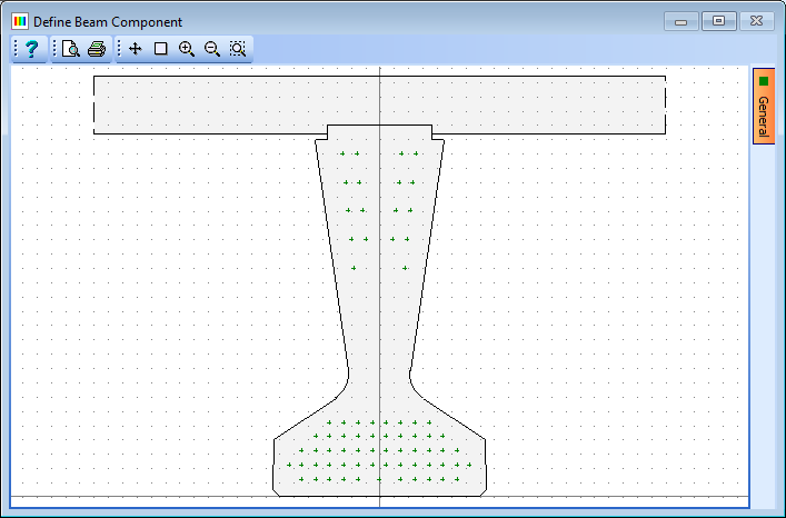
Use the Suggest size of: dropdown to select “Y Beam” which will open the Initial Sizing sub form.
On the sub form set the Beams at: “2000 centres” and select the “Y7” beam type.
Click ✓ OK on the sub-form.
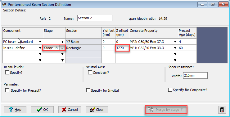
Select “Section 1” in the Define field and add an “In situ – regular” component in the second row of the table of width 2000 x depth 200mm.
Click ✓ OK on the sub form and ensure that the Z offset of the slab is 1270mm.
Click the Merge by stage # button and click on the vertical edges of this slab component to ensure that it is continuous.
Also check that the Stage for the slab is set to “Stage 1A”.
The Concrete Property for the beam and slab should be C50/60 and C32/40 respectively. Close the section definition form with ✓ OK.
For “Section 2” the program assumes the same section as section 1 so just change Stage for the slab to “Stage 1B”. Note that for both beams the age of the precast concrete is 4 days at transfer and 60 days when it is made composite with the slab.
Click ✓ OK on the Pre-tensioned Beam Section Definition form.
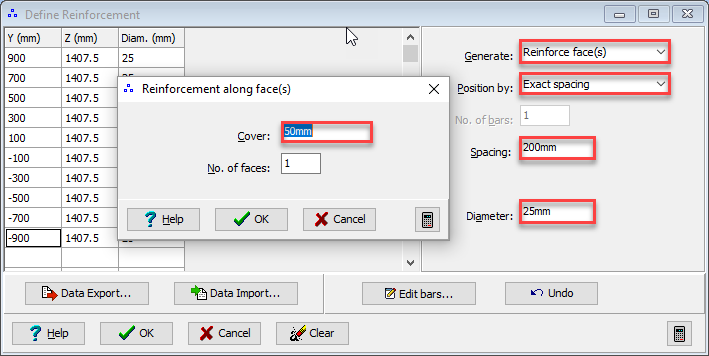
To define the reinforcement, select “Reinforcement” in the Define field.
Click the “+” button near the bottom of the form to open the Define Reinforcement form.
Set the fields to those as shown on the right-hand part of the Define Reinforcement sub form and define the cover as 50mm when clicking on the top face of the slab to define the bars.
Close the Define Reinforcement sub form with ✓ OK.
On the Define Pre-Tensioned Beam Reinforcement form, highlight all 10 rows in the table () and click on the Edit icon near the bottom of the form to open the Edit Reinforcement Attributes form.
Tick the Modify? tickbox and enter “15” in the Dimension/Start field.
Close both the Edit Reinforcement Attributes form and the Define Pre-Tensioned Beam Reinforcement form with ✓ OK.
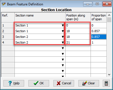
Select “Section Locations” in the Define field and set the values as shown below in the Beam Feature Definition sub-form.
Close this sub-form and the Pre-tensioned Beam Definition form with ✓ OK.

Parameters that affect differential temperature calculations and time dependant effects are also stored with the beam data so these can be defined now
In the Design Beams navigation window, select the defined prestressed beam and then click on the toolbar Analysis button to open the Pre-tensioned Beam Analysis form.
Click on the Analyse for drop down and select “Differential temperature primary stresses” to open the Differential Temperature Analysis sub form.
Set the Type of Deck field to “Type 3b: concrete beams”, the Surfacing field to “Surfaced” and the surface thickness to “0.075mm”. The resulting diff temp profile can be seen in both the table and the graphic.
Close this form with ✓ OK.
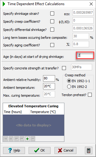
Click on the Set parameters for drop down and select “Time dependent effect calculations”.
On the Time Dependent Effect Calculation sub form set the value in the Age (in days)... field to “2” and ensure that all the other values are set to those shown below.
Click ✓ OK to close this sub form.
Finally, click ✓ OK to close the Pre-tensioned Beam Analysis form.

It is now necessary to copy and modify this beam to create the three other beams.
With the first beam selected right mouse click in the navigation window to Rename this beam “Inner Beam Span 1”.
Right mouse click again and select Copy from the list of options.
Right mouse click again and select Reverse to reverse the direction of the in-span features.
Right mouse click yet again to Rename the new beam “Inner Beam Span 2”.
To create the north edge beam of span 1, first copy “Inner Beam Span 1 and then open the Beam Definition form for the new beam.
Change the Location to “Exterior Beam”.
Open the section definition for “Section 1” and make the following changes:
1. Change the Y7 Beam to a YE7 beam.
2. Change the In-situ slab to a 1500 by 200 section
3. Change the y offset for the slab to 250
4. Define an additional In-situ regular section (Stage 2) 200 by 500
5. Set the offsets for this parapet to (-600, 1270)
6. Merge by stage #
7. Do the same for Section 2 where necessary
Delete the two reinforcing bars that are now outside the boundary of the section.
Rename the beam as “Edge Beam Span 1”.
The north edge beam of span 2 can be created by simply copying “Edge Beam Span 1”, reversing it and renaming it.
For completeness the differential temperature profile for each of the edge beams needs modifying to take into account the parapet edge. This is done by changing the profile Type to “User Defined” and then adjusting the table values as shown below:


0	15.65	0	-9.5
0.3	15.65	0.3	-9.5
0.45	3.5	0.55	-0.6
0.7	0	0.75	0
1.595	0	1.32	0
1.77	2.3	1.52	-0.9
0	0	1.77	-6.55

Line Beam Analysis of Construction Loads

In the main menu select Data | Structure Type | Line Beam.
In the Structure Definition navigation window click on the Structure Geometry icon to open the Line Beam Geometry form.
Set the number of spans to “2” and set all Span Length and Divide Span into fields to a value of “21”. The default support conditions are as required so close the form with ✓ OK.
In the Section Properties navigation window, click on the button and select Design Beam from the list to open the Structure Properties: Beam form.
In the Beam Reference field use the dropdown to select “Inner Beam Span 1” and set the Type: field to “Transformed section”.
Set the value in the Cracked Section/Proportion/from right field to “0.15”.
Click on the left-hand span on the beam elevation and click ✓ OK to assign the beam and close the form.
Repeat the previous step but select “Inner Beam Span 2” to assign the appropriate beam to the right-hand span (remembering to set the value in the Cracked Section/Proportion/from left field to “0.15”).
In the main menu select Data | Automated Loading... to open the Automated Loadings form.
Click on the Dead and SDL Loading tab and un-tick the Analyse for SDL tick box.
Select “Stage 2 Concrete” in the Continuous from Stage field and tick the Analyse for Diff Temp and Analyse for Shrinkage tick boxes.
Click on the Analyse button to carry out the load optimisation.
When this has completed click on the Transfer Results... button.
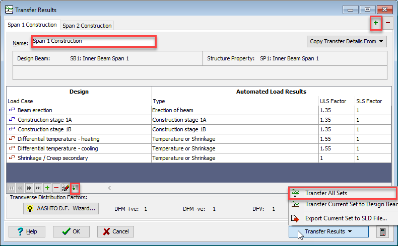
Click on the left-hand span and change the Name: field in the Transfer Results form to “Span 1 Construction”.
At the bottom of the table click on the Set Default Mapping button to create a mapping between the analysis load results and the design beam load tables.
Create a second transfer set by clicking on the + button at the top of the form and then clicking on the right span in the graphics window.
Set the Name: for this second set to “Span 2 Construction” and then carry out the automatic mapping again.
Click on the Transfer Results button and select “Transfer All Sets” from the list.
Exit the Transfer Report form and the close the Transfer Results form using ✓ OK.
In the Design Beams navigation window it can be seen that all the construction load cases and the differential temperature/shrinkage cases have entries for the two Inner beams.

Before saving the project, all the design beams should be changed to linked beams (which will save the beam data into .sam beam file and create links to them). This is not absolutely necessary but advisable as we are going to use the same beams in two different analysis projects (line beam and grillage) so any changes made by one project will automatically be seen by the other.
In the Design Beams navigation window click on the beam “Inner Beam Span 1, right mouse click and select Link from the dropdown list.
Save the file as “My EU Example 10_1 Inner Beam Span 1.sam”.
Repeat this for the other beams, saving with appropriate names.

The design beam task Embed All Linked Beams could have been used to link all the files in one go, but generic names would have been created for the file names which may not have been suitable. Further linking and embedding could use this method as the filenames now form part of the beam data.
The Line beam project file can now be saved using the main menu File | Save As... naming the file “My EU Example 10_1 Line Beam Inner.sst”.

Grillage generation
Change the analysis type for a grillage using the main menu Data |Structure Type | Refined Analysis... This will delete all the structure data for the line beam, which is intended, so accept the confirmation request.
Use the main menu item File | Titles... to change the Project Title to “2 Span Prestress Grillage” and close the Titles form with ✓ OK.

All the material and design beams are already defined but for the grillage it is necessary to define two Design Sections, one to represent the concrete transverse diaphragm and the other to represent a nominally flexible member that will be situated along the edge of the deck.
In the Design Sections navigation window toolbar click on the button and select New Section | Parametric Shape to open the Define Section Element form.
Set Width to “600”, Depth to “1470” and the Property to C32/40 concrete.
The Hook Point | Reference should be set to “-1” and the Y&Z coordinates to “0” and “0”.
Close the Define Section Element form with ✓ OK.
Rename the SS1:Section to “Diaphragm” using the right mouse button menu.
In the Design Sections navigation window click on Design Sections, at the very top, and then click on in the toolbar to add a new parametric rectangular section.
Set Width to “10”, Depth to “10” and the Property to C32/40 concrete.
The Hook Point | Reference should be set to “0” and the Y&Z coordinates to “0” and “1370”.
Close the Define Section Element form with ✓ OK.
Rename the SS2:Section to “Nominal”.
In the Structure Definition navigation window toolbar click on the button and select “Design line” to open the Define Design Line form.
Click the “+” button.
Select the Line radio button and click the “Next” button twice.
Enter (-1, 6) for the co-ordinates of point 1 and (45, 6) for point 2.
Click Next and ✓ OK twice to close all the forms.
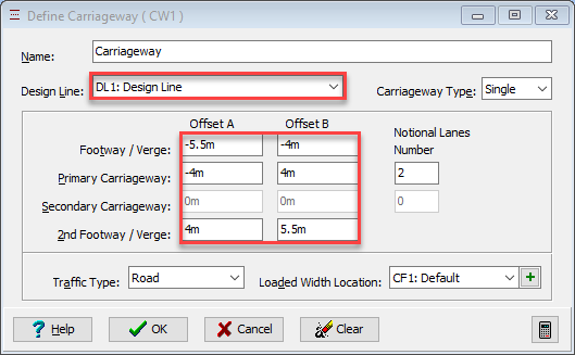
Click on the button and select “Carriageway” from the dropdown list to open the Define Carriageway form.
Set the fields to the selections and values shown below. (Note that the traffic flow direction is indicated by a triangular arrow head in each notional lane and clicking on each of the arrows until they are double-headed will show that traffic can flow in either direction. However, in this example we will leave the lanes as single direction).
Click ✓ OK to close the Define Carriageway form.
Add another Design Line with the co-ordinates (0, 0) for point 1 and (2, 12) for point 2.
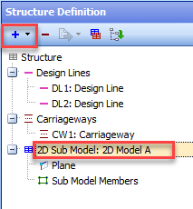
Click on the button and select 2D Sub Model (GCS, Z=0) from the list to create a new sub-model.
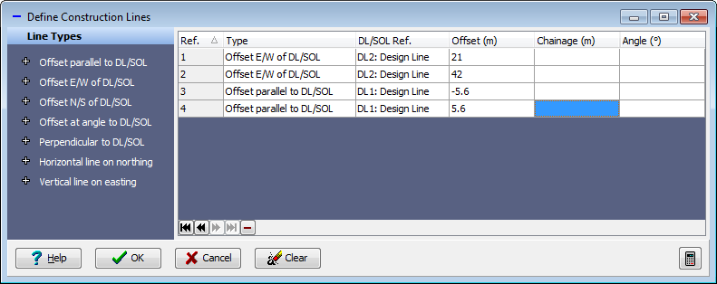
Select the sub-model, as shown below, and then click on the button to select Construction Lines which will open the Define Construction Lines form.
Use the Offset Line Types to enter the selections and values shown below.
Click ✓ OK on the Define Construction Lines form.
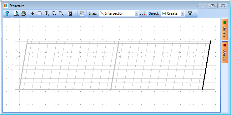
Click on the 2D Model A sub-model then click on the button and select “Mesh” from the dropdown list. This opens the Define Mesh form.
Set the Mesh Type to “Skew”.
Click on the four edges of the left-hand span, starting with the bottom edge.
Set the Longitudinal Number to “8” and the Transverse Number to “13”.
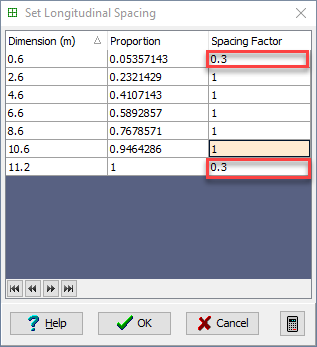
Select “set spacing” in the Longitudinal field to open the Set Longitudinal Spacing sub form.
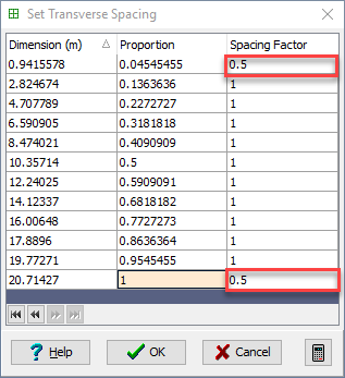
Set the values in this sub form to those shown below. Select “set spacing” in the Transverse field to open the Set Longitudinal Spacing sub form.
Set the values in this sub form to those shown below. Set the Name to “Span 1” and click ✓ OK on all the forms.

Set Longitudinal Spacing

Set Transverse Spacing
Click on the 2D Model A sub-model then click on the button and select “Mesh” from the dropdown list again.
Click on the four edges of the left-hand span, starting with the bottom edge then click on the Copy Mesh Details From button and select the first mesh to give the same mesh spacing.
Set the Name to “Span 2” and close the form with ✓ OK.
Select Structure at the top of the navigation window, click on the toolbar button and select Span End Lines to open the Define Span End Lines form.
Click on the bottom left and top left-hand corners of the structure on the graphics window. This will draw a heavy black line.
Repeat this for the central row of supports and the right-hand abutment to define the span end lines as shown below.
Click ✓ OK to close the form.
Select Structure at the top of the navigation window, click on the toolbar button and select Supported Nodes.
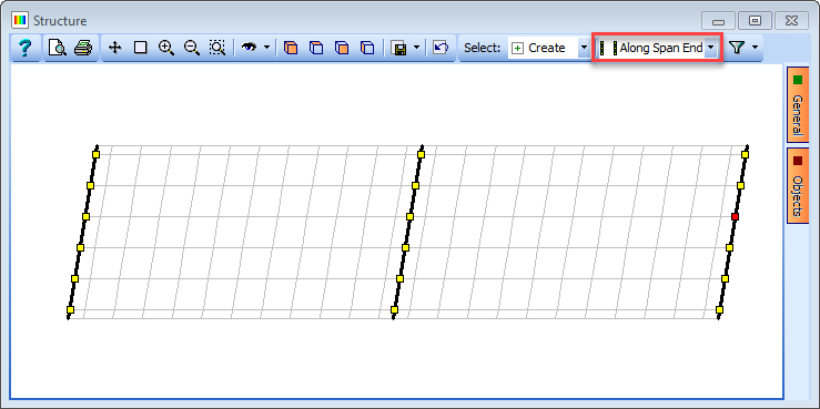
Ensure that the Select: field is set to “Along Span End Line” and select the nodes shown below.
With the Group Type set to “Uniform” set all restraints to “Free” except Direct Restraint Z, which is “Fixed”.
Now set the Group Type to “Variable” and click on the node just above the centre of the left-hand abutment.
Adjust this to be “Fixed” in the X and Y directions, then select the node just above the centre of the right-hand abutment and adjust this to be “Fixed” in the Y direction.
Click ✓ OK to close the form.

Grillage Section Properties
In the Structure Properties navigation window click on the Create Section and Beam Groups task to create one instance of each of the Design Beams and Design Section previously defined.
Select SP3: Inner Beam Span 1 in the navigation tree to open the Structure Properties: Beam form for this Beam Reference.
Change Type: to “Transformed section”, and Beam Section Reference Axis Relative to: to “origin”.
The concrete beams are to be cracked for 15% of their length either side of the central support, so set the value in the Cracked Section from right/Proportion field to “0.15”.
In the graphics window select the four inner beams in the left-hand span.
Click on ✓ OK to close the form.
Follow similar procedures to those in the previous step to assign the appropriate section properties to the other beams.
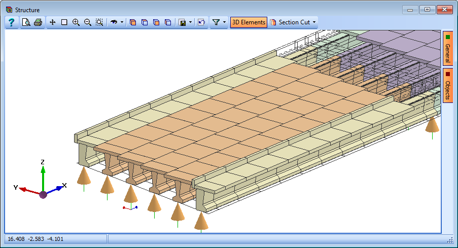
Click on the Show 3D Elements view icon in the main toolbar to view the elements of the structure in a 3D representation.

It should be noted that the south edge beams are back to front. This can be corrected by swapping the property assignments and changing the orientation of the longitudinal beams.
In the Structure Properties navigation window select SP5: Edge Beam Span 1 and then assign this to the south edge beam of span 2 (Yes to overwrite).
Also do the same for SP6: Edge Beam Span 2 assigning it to span 1.
The direction of beams can be altered in the Structure Definition navigation window by selecting Longitudinal Beams. This opens the Longitudinal Beams form.
Select the two southern edge beams (holding the <Ctrl> key for multiple selections) and select “Reverse Order_” in the _Beam Tasks list. The orientation of each beam is denoted by the small red arrow at the end of beam.
Click ✓ OK to close the form. Check the 3D Elements view again.
In the Structure Properties navigation window select SP2: Nominal to open the Structure Properties: Section form.
Assign this section to the longitudinal members at the extreme edges of the deck and change Section Reference Axis Relative to: to “origin” before closing the form with ✓ OK.
Select SP1: Diaphragm in the navigation window, set the Reference Axis Relative to: field to “origin” and assign this to the three transverse diaphragms before closing the form.
Click on the button and select “Continuous slab” from the dropdown list. This will open the Structure Properties: Continuous Slab form.
Change the Depth to “200mm” and Description to “Transverse Slab” and ensure that the Material Property is the grade “32/40 property.
Click on the Member selection filter dropdown menu and select “Transverse Beams”.
Draw a box around the whole structure and answer “No to All” on the confirmation box that appears. This stops the program form overwriting the diaphragm section assignments.
Now remove the filter by clicking on the Member selection filter drop down and selecting “Select All”.
Click on ✓ OK to close the form.
Click on the 3D Element View icon to view the elements of the structure in a 3D representation. Note that the transverse slab members are incorrectly located at the soffit of the pre-cast beams.
In the Structure Definition navigation window, click on the "+" button and select Advanced Beam Set | Eccentricities form the dropdown list to open the Define Beam Eccentricities form.
Click on the “+” button to add a row in the table and enter a value of “1370” in the Start Z and End Z columns.
Apply this eccentricity to the transverse slab members which can be achieved by opening the filter form to first Deselect all and then Select By “Structure Property” where just the “Transverse Slab” property is selected before closing the filter form.
Drawing a window round the whole structure will then apply these offsets to just the slab members.
Close the Beam Eccentricities form with the ✓ OK button.
Set the filter to “Select All” before using the 3D Element viewer to check the outcome of these changes.

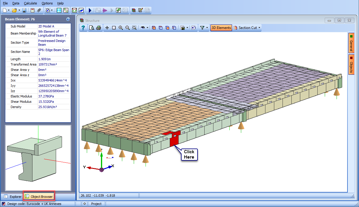
Note that the members are now correctly located. Clicking on the Object Browser tab below the Navigation Pane and selecting an element in the graphics window displays detailed information about that element in the space that is normally occupied by the Navigation Pane.

Grillage Basic Loading

The next step is to apply some basic superimposed dead and live loads to our model, (the dead loads for concrete have already been input into the beam files by means of transfer from the Line Beam module).
In the Structure Loads navigation window click on the toolbar button and select Bridge Deck Patch Load from the drop down list to open the Define Bridge Deck Patch Loading form.
Set Load per unit area to “2kN/m²” (press the enter key to register it).
On the graphics window, move the mouse pointer over the Objects tab and deselect “Design / Setting Out Lines”, “Construction Lines” and “Beam Elements” (click on the Objects tab if it does not open when the mouse pointer is moved over it). The graphics now shows the carriageway and span end lines.
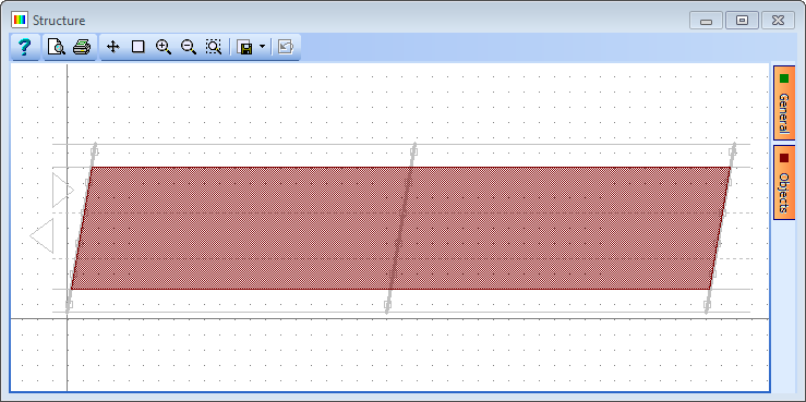
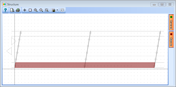
Click on the bottom edge of the main carriageway, the right hand span end line, the top edge of the carriageway and the left hand span end line (See the screen shot on the following page for details of the carriageway edge locations). This will apply a patch to the carriageway.
Change Name to “SDL – Carriageway”.
Click ✓ OK to close the form.
Create a second Bridge Deck Path Load with a Load per unit area of “3kN/m²”.
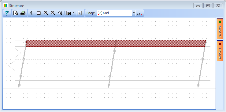
Click on the bottom edge of the south verge, the right hand span end line, the top edge of the south verge and the left hand span end line. This will apply a patch to the south verge.
Change Name to “SDL – South Verge” then click ✓ OK to close the form.
Repeat the process for the north verge to assign a Bridge Deck Patch Load of 3kN/m² as shown below.

The next step is to define an SDL barrier load.
On the graphics window, move the mouse pointer over the Objects tab and select “Beam Elements”.
Click on the button and select Beam Member Load | Beam Element Load from the drop down list to open the Define Beam Loading form.
In the first row of the table set Load Type to “F Uniform”, Direction to “Global Z”, Load Value to “Length” and Load W1 to “-1.3kN/m”.
On the graphics window, click on the filter drop down and select “Longitudinal Beams”.
Draw boxes around the edge longitudinal beams to assign the loads.
Press <Ctrl-A> on the keyboard to remove the filter.
Change Name to “SDL - Barriers” and click on ✓ OK to close the Define Beam Loading form.

The next step is to create SDL compilations for ULS and SLS.
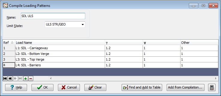
In the Structure Compilations navigation window click on the toolbar button and select Superimposed Dead Load to open the Compile Loading Patterns form.
Set the Limit State field to “ULS STR/GEO” and click the Find and Add to Table button to add all the basic loads into the table.
Change the Name to “SDL ULS” and click on ✓ OK to close the form.
Right click on compilation “C1: SDL ULS” on the Navigation Pane, then select Copy to create a duplicate of the first compilation.
On the Compile Loading Patterns form, change Limit State to “SLS Characteristic” and click on “Yes” in the confirmation dialog.
Change the Name to “SDL SLS” and click on ✓ OK to close the form.

Grillage Traffic Load Optimisation

The next task is to create some influence surfaces and generate live load patterns using the load optimisation in the program.

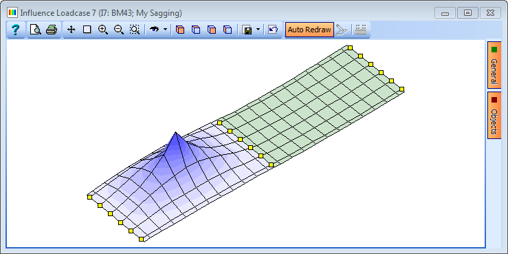
The first step is to define the influence surfaces we want to generate, which are bending moment influences at each point along one inner beam in span 1.
In the main menu select Data | Influence Surface to open the Influence Surface Generation form.
Set Pick Mode to “Longitudinal Beam” then click on the inner beam located just above the centre of the deck in the left-hand span in the graphics window. This will define 13 influence surfaces for My Sagging.

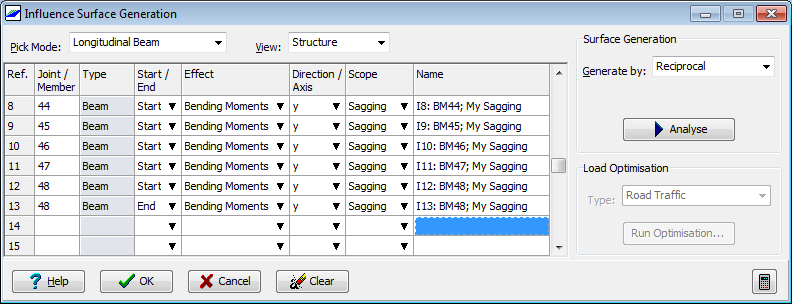
The next step is to analyse the structure to generate the influence surfaces.
Set Generate by to “Reciprocal” and click on the Analyse button. A progress box will open.
Click on the ✓ Done button when the analysis has completed. The graphics window will now show the influence surface for the first member selected.
Change the view to isometric then click the first line in the Name column on the Influence Surface Generation form.
Use the up and down cursor keys on the keyboard to move through the influence surfaces.

For each influence surface an optimised traffic load pattern can be created for different types of Eurocode load combination. Each load pattern is defined as an ASBD load compilation.
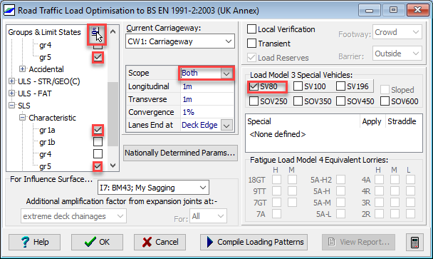
Set Type to “Road Traffic” then click on the Run Optimisation... button to open the Road Traffic Load Optimisation form.
In the Groups and Limit States area click on the button and select “Clear All” before expanding the ULS-STR/GEO (B) and SLS Characteristic groups to select both gr1a and gr5 in each.
As the gr5 combination has been selected it is necessary to specify the type of Load Model 3 Special Vehicle(s) which in this case should be SV80 only.
Ensure that the Scope field on the Key data tab is set to “Both” to ensure both sagging and hogging load patterns are generated.
Click on the Compile Loading Patterns button to run the load optimisation.

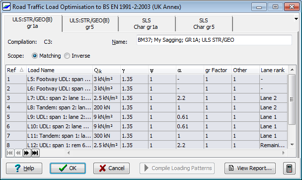
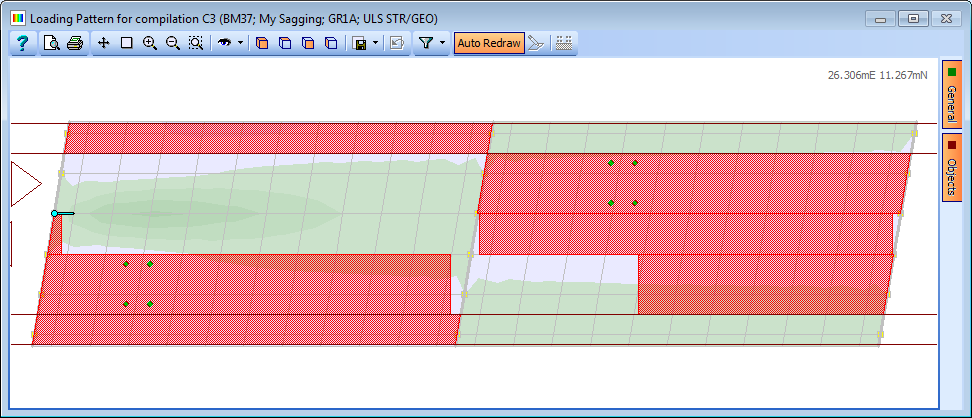
Details of the load optimisation run will be shown together with the loads created both on the form and in the graphics window. (2 notes may appear on the Results Viewer regarding the SV80 influence surface which are for information and can be ignored i.e. close the results viewer).
Use ✓ OK on the load optimisation forms to close it and save the loads and compilations that have been created.

With some small modifications the data in the influence table can be used to create influences for shear force.
In the first row of the Effect column, change “Moment” to “Shear Forces” and respond with “Yes” when asked if all other points below this are to be changed.
In the first row of the Start/End column change “Start” to “End” and then delete the very last row in the table (it is not possible to use the reciprocal method for shear at nodes that are supported).
Click on the Run Optimisation... button to open the Road Traffic Load Optimisation form and then click on the Compile Loading Patterns button to run the load optimisation as all the parameters are the same.
In the confirmation window select “No” to deleting the previously generated loads.
Use ✓ OK on the load optimisation forms to close it and save the loads and compilations that have been created and also close the Influence Surface Generation form with ✓ OK.

The next task is to solve all the load cases.
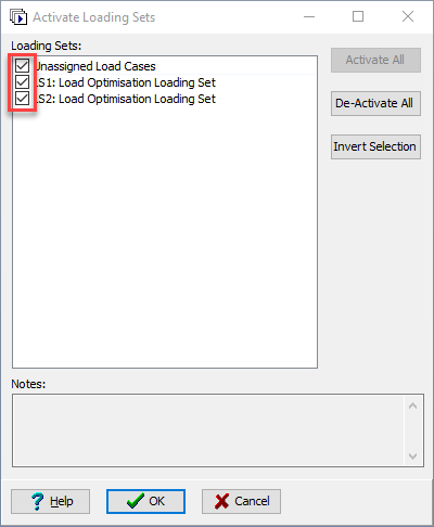
In the main menu select Calculate | Analyse Structure... where the Activate Loading Sets form will open. This allows you to select which loading sets you want to solve. Each time the load optimisation is run, a new loading set is automatically generated for the load cases produced by that run so in this case there will be two cases. The list also includes any load cases not included in a loading set (as Unassigned Load Cases).
Make sure all tick boxes are ticked and click ✓ OK.
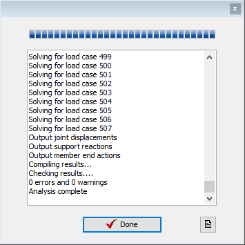
The program will open a form showing the progress of the analysis. Once the analysis has completed, click on the ✓ Done button.

It is good practice to inspect the results produced in the analysis, to check that they make sense, before transferring them to the design beam load tables.
In the main menu select File | Results... to open the Results Viewer.
Click on the Result Type drop down and select “Compilation” from the list of options.
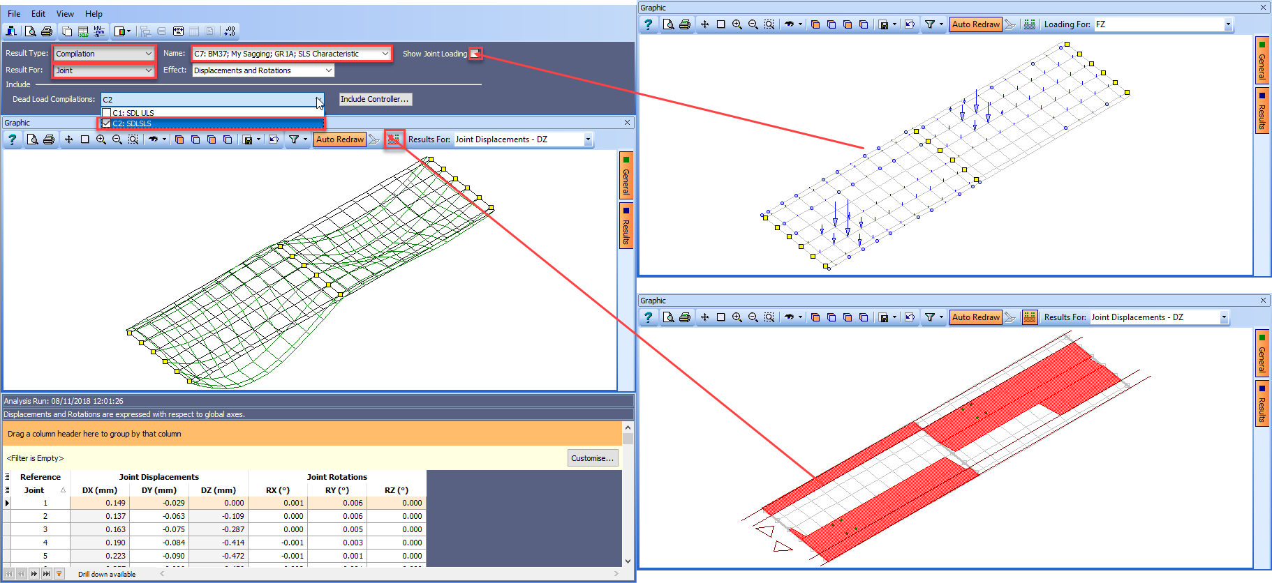
In the Name dropdown select compilation C7 (which is an SLS compilation), set the Result for to “Joint” and Effect to “Displacements and Rotations”.
It is required to inspect the results with other permanent load effects at SLS added. (Note that in this model we can only add in SDL because the self weight of the concrete is only included in the individual Pre-stress beam files). Click on the Dead Load Compilations dropdown and tick C2. This will add the effects of this compilation to compilation C7 and show the displacements for the load cases in the two compilations applied together.

The load pattern causing this displacement can also be displayed by clicking on the icon in the graphics toolbar, as shown, and the resolved nodal loads from this loading displayed by ticking Show Joint Loading. Filtering can be applied to limit the results to certain parts of the structure, for example, a line of edge members.
Click on the Result For dropdown and select “Beam” from the list.
In the Name field, select compilation C6.
Click on the Filter toolbar to open the Member Selection Filter form.
Click on De-select all then set Pick Mode to “Longitudinal Beam”.
Change the graphics view to plan and click on the bottom edge beam in span 1.
Click on ✓ OK to close the filter form and change the view back to isometric.
The graphics now shows a plot of the Z member end forces.

We can also overlay a bending moment diagram on the plot.
To do this, click on the Results for dropdown menu on the graphics toolbar (not in the header). You will see tick boxes next to each result type with Fz already ticked.
Tick the My option as well to add the bending moment diagram to the plot.
The scale is a bit small for the plot so move the mouse over to the Results tab on the right hand side of the graphics and tick both the Specify Scale tick boxes.
Enter values of 10kN and 50kNm in the two boxes. The Results Viewer will now look like this:

We can also look at the joint displacements for all compilations for the centre joint of span 1.
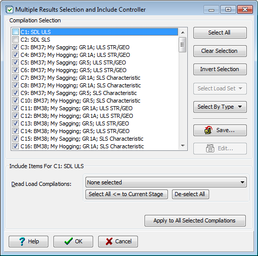
To do this, change Result For to “Joint” then click on the Edit | Multiple Results Selection menu item. This will open the Multiple Results Selection and Include Controller form.
Click on the “Select All” button then un-tick the first two compilations.
Click on ✓ OK to close the form and display the displacements for the selected compilations. All the displacements are there but they are grouped by compilation.

If it was required to establish the max negative DZ displacement for one particular node over all live load compilations (without having to create an envelope), say node 46, then the table could be ungrouped and the table sorted so the max was at the top.
Drag Including Dead Load Compilations and Compilation Name off the orange bar to ungroup the results.
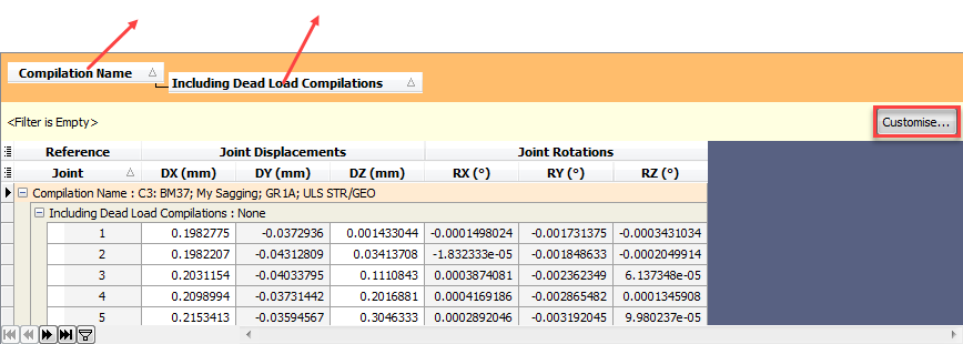
Click on the Customize... button at the top right of the results table.
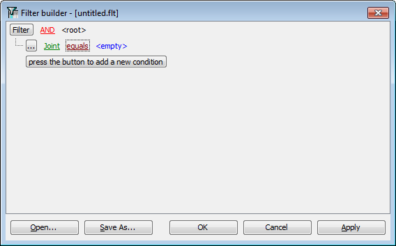
On the Filter Builder form click on the button marked press the button to add a new condition then click on the green text and select “Joint”.
Click on the blue text which says 'empty' and type “46” then click on the ✓ OK button.
Set the Results For: drop down menu on the graphics toolbar to “Joint Displacement-DZ”.
Click once on the DZ column header to sort the list from low to high, then scroll to the top to see the maximum negative displacement for joint 46.
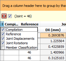
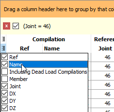
To see which compilation produces this displacement, additional columns can be added to the table. Click on the menu option to the left of the Reference heading in the results table.
Tick “Compilation” then click on the menu below and tick “Name” and “Ref”.

Ref Name Results

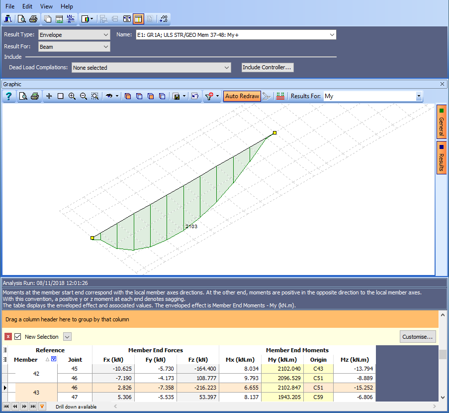
The load optimisation was carried out for one longitudinal beam so the program automatically created bending moment envelopes for that particular beam.

To see these enveloped results, click on the Result Type drop down and select “Envelope”. The Name field should show envelope E1.
Click on the Filter button then De-select all, set Pick Mode to “Longitudinal Beam” and click on the inner beam just above the centre of the deck in span 1 on the screen.
Click on ✓ OK to close the filter form.
Put your mouse over the Results tab on the right of the graphics and untick the two Specify Scale tick boxes.
Put your mouse over the General tab and tick the Result tick box. This will show the maximum My moment.
Finally, close the Results Viewer.

Transfer Grillage Results to Beam File

The analysis results can now be transferred to the pre-stress concrete beam design load effects tables. There are three basic methods of transferring results that can be chosen for this example.
- Embed the linked beam and transfer the results to the beam tables in the current project
- Transfer the results directly to the linked beams which will update the linked beam files
- Transfer the results to an intermediate ASCI .sld file which can then be imported into the beam tables at a later time
In this example the first method will be used so that the resulting tables can be seen instantly and design checks carried out in the project. The embedded design beam can then be linked to the existing beam file which will of course be updated with the current data. This will ensure that any other project linked to this file (eg the line beam analysis, saved earlier) will automatically see these changes.
In the Design Beams navigation window select the linked beam “Inner Beam Span 1” then in the navigation toolbar click on the unlink icon to break the link and embed the data.
In the main menu select Calculate | Transfer Results ... to open the Transfer Results form.
In the graphics window click on the inner beam just north of the centre of the deck in span 1. It will be highlighted in red. It is now required to match envelopes/compilations produced during the analysis with design load cases in the Design Beam.
Starting with SDL cases, add two lines of data using the “+” button at the bottom of the table.
In the Design | Load Case column select “Surfacing 1” in both rows.
In the Type column select “Compilation” in both rows and in the Structural Analysis | Load Case column, select SDL ULS in the first row and “SDL SLS” in the second. The Factors will be automatically set to 1 in the appropriate column.
Change Name: to “SDL Inner Beam Span 1”.
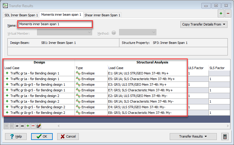
Create an additional transfer set by using the "+" button at the top right of the form, select the same beam in the graphics and change the Name: to “Moments inner Beam Span 1”.
Add eight lines of data using the “+” button at the bottom of the table as there will be four sagging cases and four hogging cases and select entries in each field as shown below:
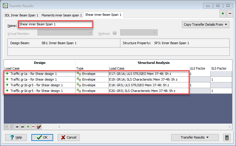
Create an additional transfer set and change the Name: to “Shear inner Beam Span 1”.
Add four lines of data using the “+” button at the bottom of the table as there will be four shear envelopes and select entries in each field as shown below:
Click on the Transfer Results button and select “Transfer All Sets” to transfer the results to the beam design tables.
Use ✓ OK to close the Transfer Results form.

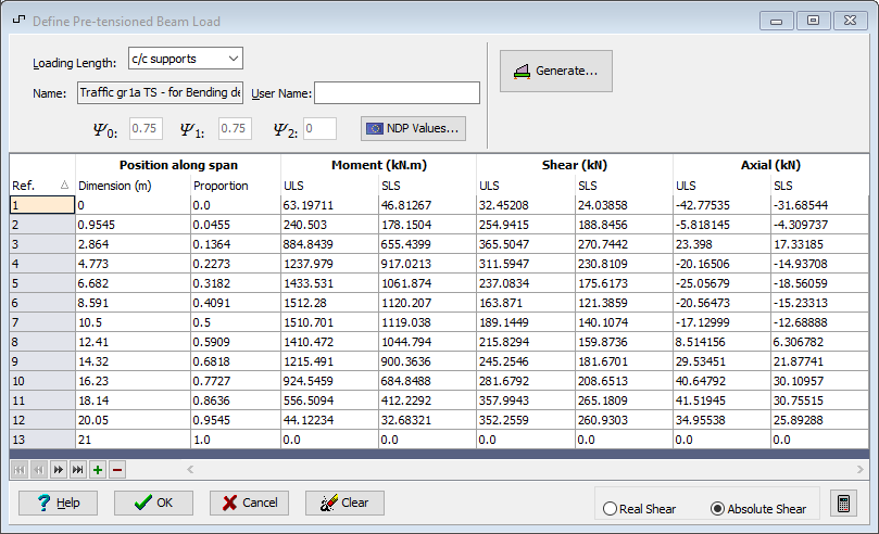
In the Design Beams navigation window it can be observed that all of the Beam Loads tables are now available for inspection and subsequent code checking.

It should be noted that each of the gr1a traffic loading cases has been split into three components, one for the UDL, another for the Tandem system (TS) and the third the footway load. The reason for this is that each component may have different psi factors when combining it with other variable actions when looking at different design checks.
To display the load effects that have just been transferred, in tabular and graphical form, just click on the load table in the navigation window and it will be displayed.

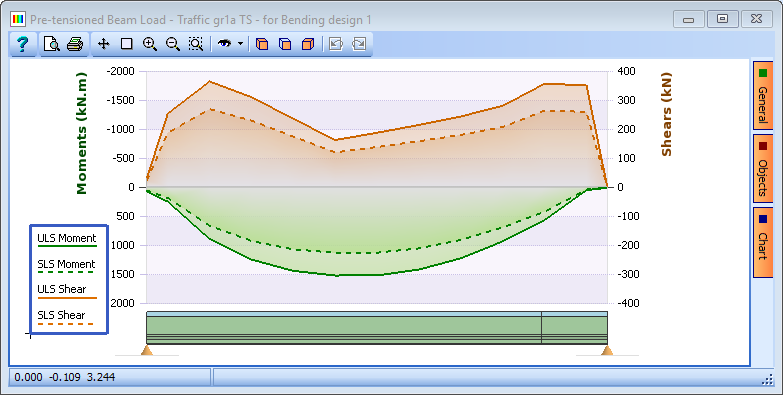
Beam Analysis/Design
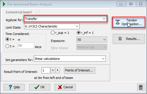
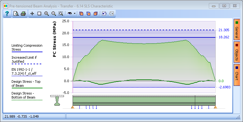
In the Design Beams navigation window toolbar click on the analyse icon to open the Pre-tensioned Beam Analysis form and then set the Analyse for: field to “Transfer”.

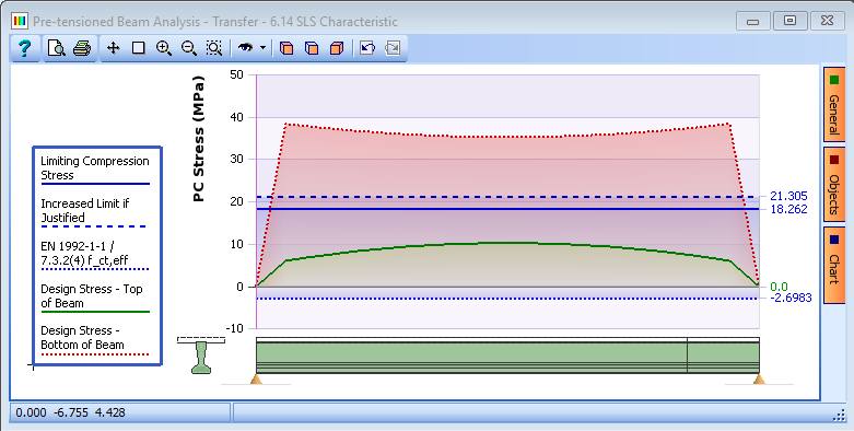
This shows that the design stresses in the bottom of the beam far exceed the limiting compressive stress for this age of concrete. There are a number of design changes that can be utilised to correct this (removing tendons, debonding tendons, changing material properties etc) but in this example the tendon optimisation can be used to see if there is a good solution by just removing and debonding some tendons.
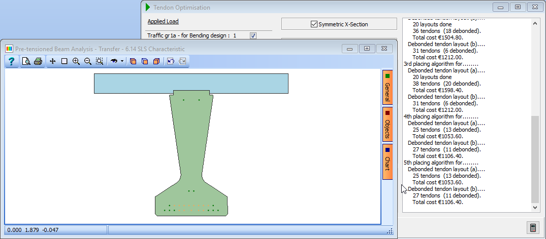
Click on the Tendon Optimisation button on the analysis form and then dismiss the information message displayed.
Tick the four Applied Load boxes and the Debond option but un-tick the Straight box.
All other default data is acceptable so click on the Design Optimised Layout button.

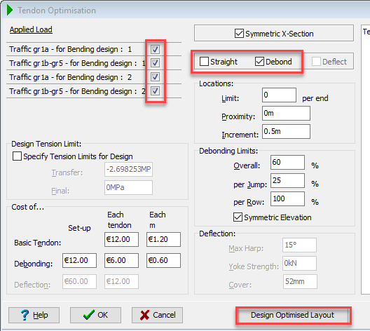
It may take a few minutes to complete the optimisation and a few warning messages may be displayed (which can be accepted).
Close the Tendon Optimisation form with ✓ OK and the affect of the optimised tendon layout is immediately obvious showing that the stresses are now acceptable.
All other design checks can then be carried out to ensure compliance with stress limits etc. by changing the various parameters on the Analysis form.

For instructions on how to carry out these various checks on the design beam, in accordance with Eurocodes, see Section 5.2 of this Examples Manual.
Once all the checks (and changes if necessary) have been made, close the Pre-tensioned Beam Analysis form with ✓ OK.
To save all Design Beam changes to the original linked Design Beam file the embedded beam can be changed to a linked Design Beam using the same name as the original design beam file. This will update the data in this file to reflect the changes made in this project.
Finally, use the main menu File | Save As... to save the project data to a file called “My EU Example 10.1 Grillage.sst” and close the program.