Optimization Constraints
Learn about optimization constraints and how to specify them.
Learning Objectives
- Use constraints as surface restrictions.
- Observe that conflicting constraints can make a problem not feasible.
- Summarize that proximity measure is a value that indicates closeness to a feasible solution and how it can be used to determine the feasibility of a problem in a convergence plot.
About Constraints
Every optimization problem consists of an input. In Grading Optimization this is an existing ground surface made up of triangles. The optimization solver will change the surface, and after completion, return a new surface. However, we do not want a random surface. From the infinitely different surfaces that the solver can create, the surface that satisfies specific criteria is desired. For example, you may want the surface at any given point to exceed a maximum slope of 33% (or 3:1 ratio). Restrictions such as this are called constraints.
A constraint in Grading Optimization is a restriction that is placed on the input surface.
Feasibility
You can place a large number of constraints on a surface. It is also possible to add a combination of constraints that conflict. Consider the following drawing depicting a building pad on a terrain.
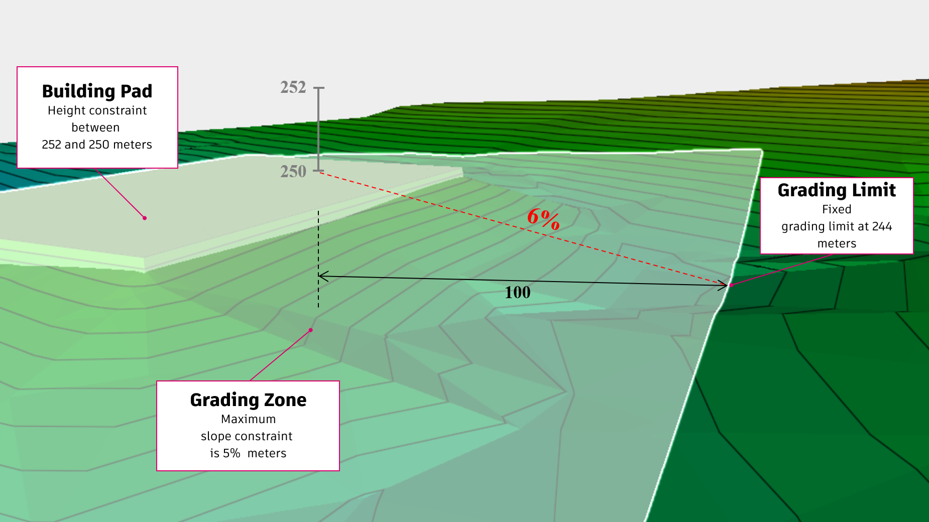
Assume the following constraints:
- A maximum slope constraint is set to 5%.
- The building pad elevation is set between 250 and 252 meters.
- The property boundary ends 100 meters from the building.
- The grading limit elevation is 244 meters.
The slope between the grading limit and the minimum building elevation is 6% which is more than the maximum slope of specified 5%. The solution for this surface grade is not feasible.
Grading Optimization can still work with an inconsistent problem and find a reasonably feasible solution. In this example, the solution could resolve where the terrain slope ends up at 5.5% and the building elevation at 249.5 meters.
A feasible problem is always solvable. If a problem is not feasible, Grading Optimization will find a best approximation.
Proximity
Grading Optimization changes surface elevations iteratively to solve for the constraints. The closer it gets to a feasible solution, the less change is needed in the surface. How much the surface needs to be changed within an iteration, to satisfy all the individual constraints, is measured by a value that we call the proximity measure.
The proximity measure is the sum of the distances between the position of the current surface points and the position where each individual constraint would require them to be.
This is best illustrated in our previous approximation example. Assume that solution is represented by the following drawing.
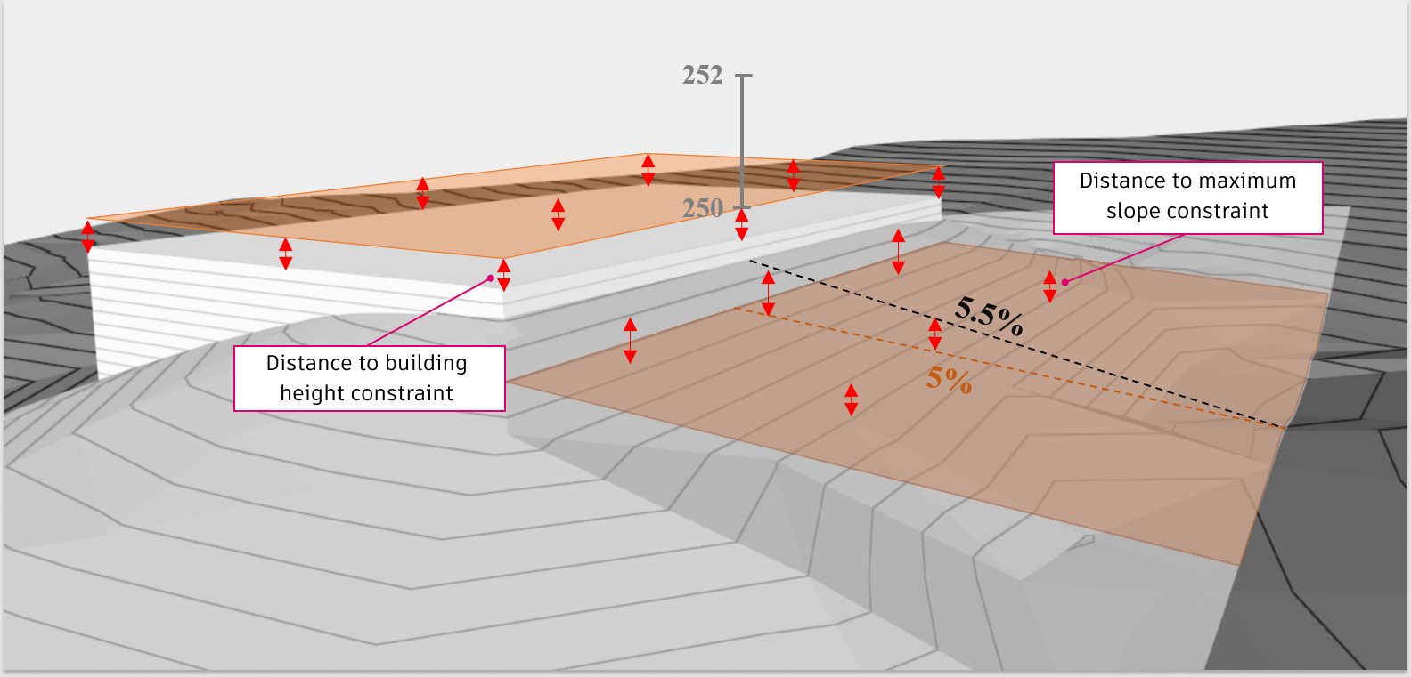
The distance between the building pad at 249.5 and the height constraint at 250 is 0.5. If there are 10 building pad points, they are each a distance of 0.5 away from the height constraint, and the sum of these points contribute a total of 10 * 0.5 = 5 to the proximity value.
Furthermore, the group of points from the triangles on the terrain that are sloping at 6% are also, a certain distance away from the desired 5% slope surface. If we assume that all the distances from this group add up to 10, then we end up with a total proximity measure of 5 + 10 = 15 for our best approximation. Since the solver cannot make this solution better, the proximity measure will remain constant at this value 15, as the iterations progress.
When a problem is feasible, the proximity measure will decrease towards zero as the iterations progress. If a problem is not feasible, the proximity value will level out at a value greater than zero.
In Grading Optimization, we can look at the proximity measure in the Feasibility part of the Convergence Plots dialog.
Click  on either the Violation tab or Cut-fill tab of the Optimization Panel to open the Convrgence Plots dialog.
The images below show the proximity measure for four different problems different problems. the first two are feasible, the second two are not feasible.
| Feasible? | Example |
|---|---|
| Yes | 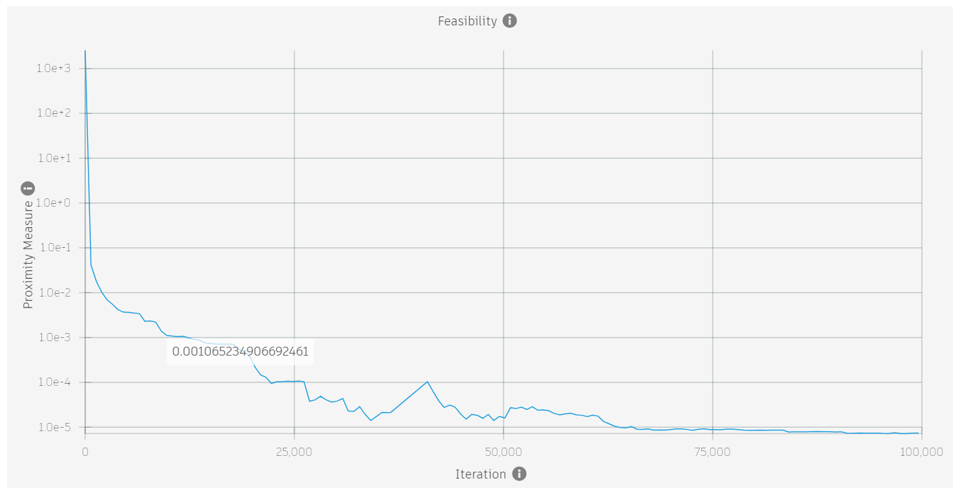 |
| Yes | 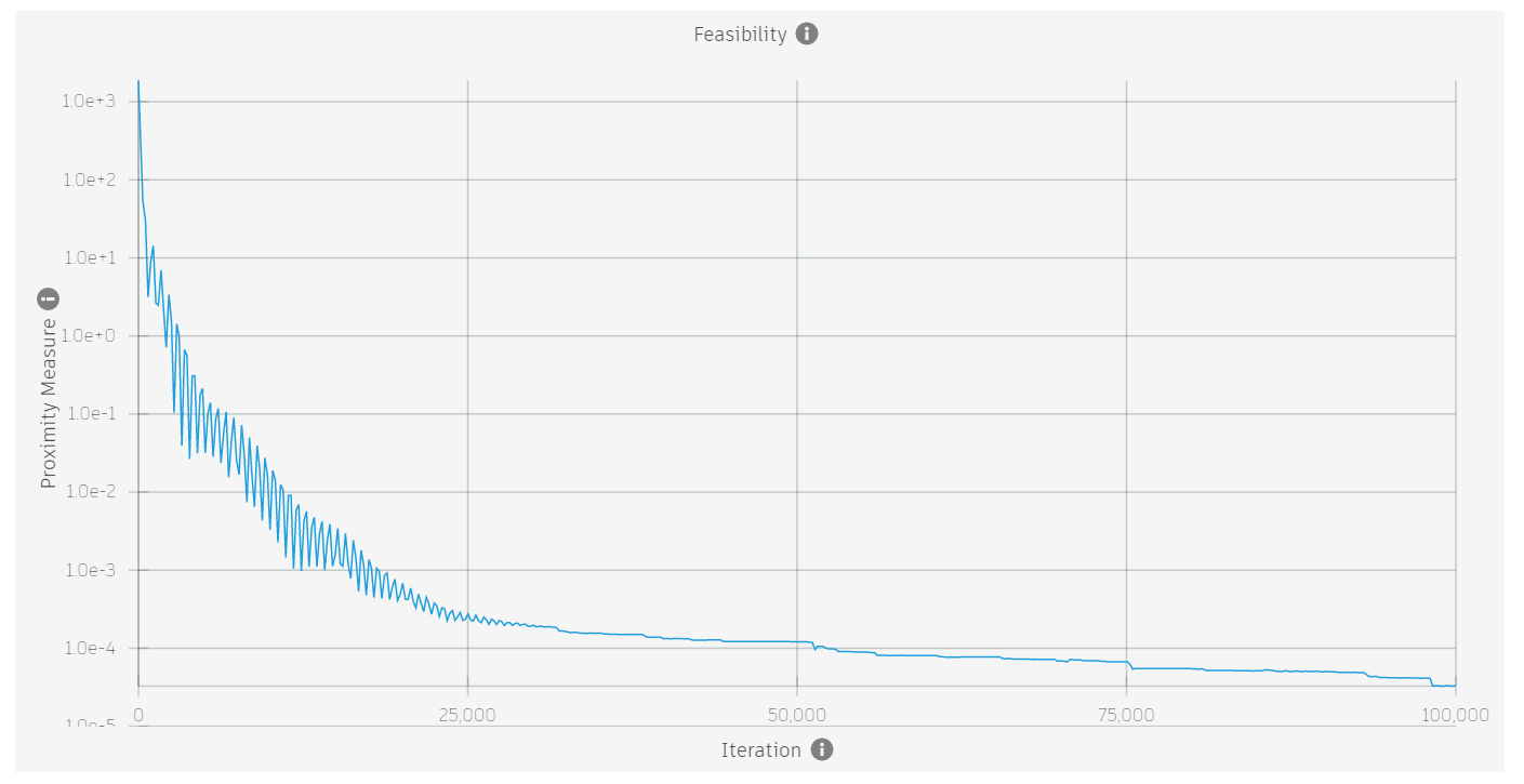 |
| No | 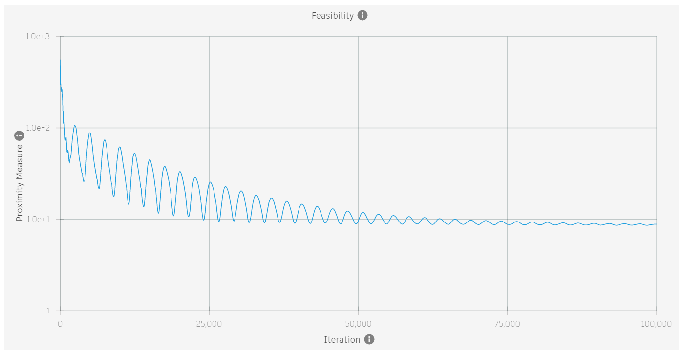 |
| No | 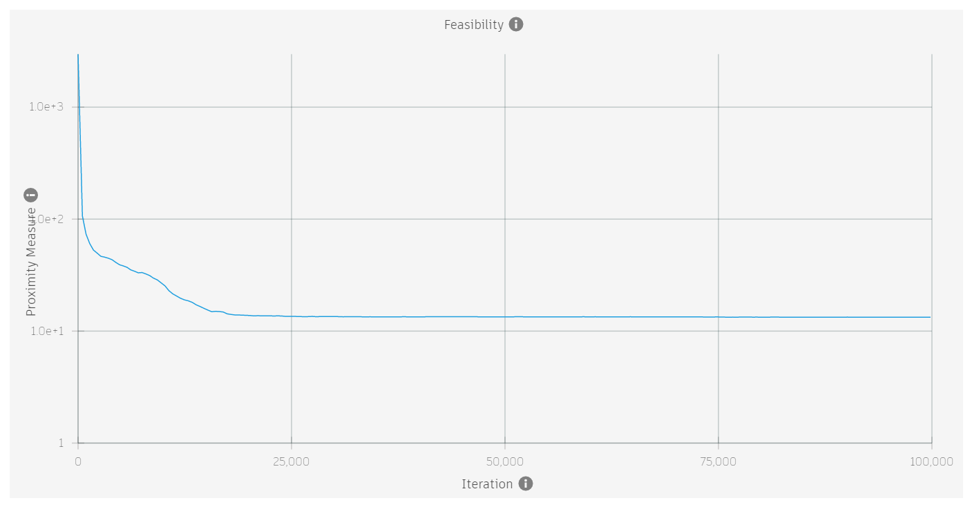 |
A typical case of an infeasible problem is when the maximum slope constraint on a grading limit zone is set to a value that is smaller than the actual slopes along the boundary of the grading limit. Since grading limit zones have fixed boundaries, the solver will not be able to satisfy the maximum slope at these locations. In such a case, Grading Optimization warns at the start of the optimization.
