The Quick-Start tutorial is designed for first-time users of InfoWater Pro Scheduler and provides a guided tour to core commands and functions used to create and execute a scheduling optimization run. The Quick Start tutorial will help you become familiar with the core set of InfoWater Pro Scheduler features and should be used as a launching point to a more comprehensive understanding of the program.
The estimated time to complete the Quick Start tutorial is approximately 30 minutes. The Quick Start tutorial will help you become familiar with the following:
- Defining control groupings.
- Setting system constraints.
- Launching a GA optimization run.
- Reviewing and analyzing GA optimization results.
- Exporting optimal time control rules for various uses.
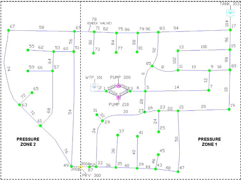
During the Quick Start tutorial, you will modify an existing project called “SampleSchedule”. This “SampleSchedule” project can be downloaded from Quick Start Tutorial Example files. The “SampleSchedule” project modified in this tutorial illustrates how InfoWater Pro Scheduler automatically identifies the optimal scheduling policy that minimizes operating cost while satisfying the desired operational requirements of the system. The “SampleSchedule” model schematic is shown below. The model contains two pressure zones and consists of the following components:
- One reservoir (storage node 101)
- One tank (storage node 103)
- Two pumps located at the water treatment plant and numbered 200 and 210
- One pressure reducing valve located at node 300
- One check valve located in pipe 78
- Fifty-eight pipes
- Forty-five junction nodes
- One reference file containing the parcel and street layout (not shown in the illustration below)
Step 1: Open the Project
The first step is to open the InfoWater Pro project.
- Choose the Start menu, select Programs, choose the InfoWater Pro Version 2.5 or higher program group, and then choose InfoWater Pro.
- In the ArcMap window, select an
Existing Map option in the
Start Using ArcMap With area and then click on
OK button. If the
ArcMap window is not shown, simply choose
Open command from the
File menu: SampleSchedule.aprx.
Note: If you have not previously downloaded the Example files, you can do so from Quick Start Tutorial Example files.
- Click on the Red Down arrow
 icon to initialize InfoWater Pro. When initialized, the icons on the InfoWater Pro toolbars will be enabled for use.
- Before continuing, save the “SampleSchedule” project to a new project. If you wish to restart the tutorial, the original project will be available. Choose the Save As command from the File menu. On the dialog box, enter the new project name “Tutorial”. This becomes the active project.
- Click on the
InfoWater Pro ribbon, and then select the
Apps
 command from the
InfoWater Pro ribbon. Select
Scheduler from the
App Manager dialog box. Click on the
Run button. Choose
Simulation
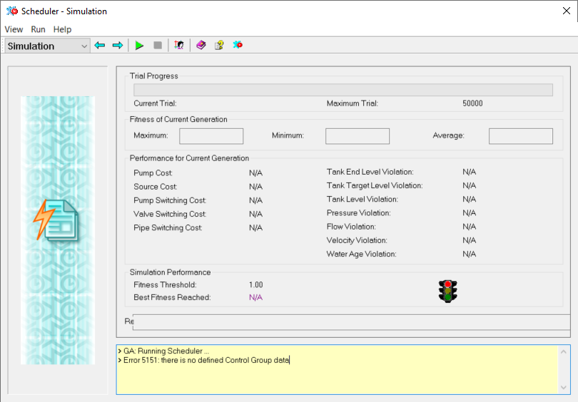
from the drop-down menu. The following dialog box appears when the InfoWater Pro Scheduler is launched from the App Manager dialog box.
command from the
InfoWater Pro ribbon. Select
Scheduler from the
App Manager dialog box. Click on the
Run button. Choose
Simulation
from the drop-down menu. The following dialog box appears when the InfoWater Pro Scheduler is launched from the App Manager dialog box.
Step 2: Create Pump Groups
The first step in the scheduling process is to define the control groupings. Here we will create pump groups. It is assumed that all pumps in a pump group will operate in an identical fashion with similar start, stop and switching times. For this example, you will create two pump groups, one group for each pump. To do this, you will add a new database field (we will call it PGROUP) to the existing Pump Information database table and populate it with the appropriate pump group IDs.
- Select the DB Edit… button to access the InfoWater Pro Pump Information Database Table.
- Choose the Edit/View Fields button and click on the Append button to add the PGroup database column entry. Select a Data Type of “Integer” and a Field Length of “4” in the Field Definition – Append dialog box as shown below.
-
Choose on the OK button and then click on the Apply button to enter your selection. The PGroup data field will be on the far right side of the Pump Information data table.
- You will now enter the pump group ID for each pump in the PGroup data field. For this example, use a group ID of “1” for pump 200 and a group ID of “2” for pump 210. After you added the pump group ID, press the Enter key to update the PGroup field.
- Select the Save button and then choose the Exit button at the top of the Database Editor and you are returned to the InfoWater Pro Scheduler dialog box.
- Choose PGroup from the Pump Group Database Field drop-down list as shown below. The pump IDs for each pump group will be displayed on the InfoWater Pro Scheduler dialog box.
Step 3: Define Pump Operational Requirements
The next step is to define for each pump group the pump operation period, the starting time, the maximum number of pump switches, and the switching time interval. Use the table below as a guide when entering this data.
| Maximum Switches | Start Time | Simulation Duration | Switching Interval | Pump IDs |
| 24 | 0.00 | 24 | 1 | 200 |
| 24 | 0.00 | 24 | 1 | 210 |
The InfoWater Pro Scheduler dialog box now appears as follows.
For this example, we will use the pump efficiency curves and energy charge pattern provided with the “Sampleschedule” project. Both pumps 200 and 210 share the same energy charge pattern but have different efficiency curves. However, no demand charge will be considered. To inspect the energy data provided for both pumps, close the InfoWater Pro Scheduler dialog box (select the Exit command from the View menu) and use the following steps:
- Click on the Select Element icon from the InfoWater Pro Edit Network toolbar, place the cursor on pump 200 and then click on the left-mouse button.
- Click on the
Tools icon on the Attribute Browser window, then choose the
Energy Pattern command. The Pump Energy dialog box appears on the screen. Click on the
Browse
 button to inspect the energy charge pattern, and then on the
Cancel button to close the Pattern dialog box.
button to inspect the energy charge pattern, and then on the
Cancel button to close the Pattern dialog box.
- Click on the Cancel button to close the Pump Energy dialog box.
- Click on the
Tools icon on the Attribute Browser window, then choose the Energy Efficiency command. The Pump Efficiency dialog box appears on the screen. Click on the
Browse
button to inspect the efficiency curve, and then on the
Cancel button to close the Curve dialog box.
- Click on the Cancel button to close the Pump Efficiency dialog box.
Repeat steps 1 through 5 for the second pump 210 and re-launch the InfoWater Pro Scheduler. Remember that both pumps share the same energy pattern yet have unique efficiency curves.
Step 4: Create a Domain
You will now define a Domain so that all the network components defined in the domain will be a factor in the InfoWater Pro Scheduler evaluation process. However, the values specified in the Constraints for Domain area will be overwritten by any values entered in the Specific Constraints area.
- Select the
Apps
command from the
InfoWater Pro
ribbon. With the Apps Manager dialog box open, select Scheduler and click on the
Run button.
- Choose the Edit Domain button on the InfoWater Pro Scheduler dialog box and the Domain Manager dialog box appears on the screen.
- In the Element Source area, select the Network option and All Elements from the drop-down list, then click on the Add button to place all the network components in the Domain.
- Click on the Close button to close the Domain Manager and to return to the InfoWater Pro Scheduler dialog box. All elements highlighted in red constitute the Domain.
You will now define the hydraulic constraints for the scheduling problem.
Step 5: Set Tank Constraints
There are several constraints that can be specified for tanks. These include minimum level, maximum level, final tank level, and a tolerance for matching the ending tank level. Final storage bounds are usually tightened (small tolerance) so that the storage in the tanks will be more or less the same as the initial states (hydraulic periodicity condition).
- Select the Tank Level Constraint option in the Input Data view category.
- For this example, you will specify in the Constraints for Domain area a 40 % minimum percent level, a 95 % maximum percent level, an end percent level of 88 %, and a tolerance of 5 % as illustrated below. No specific constraints will be defined.
Step 6: Set Junction Constraints
For this example, you will specify a minimum pressure of 40 psi and a maximum pressure of 120 psi for all the junctions specified in the Domain. However, Junction IDs 1, 3, 17, 49 and 87 will have different target pressure values and thus will overwrite the values specified in the Constraints for Domain area.
- Select the Junction Pressure Constraint option in the Input Data view category. In the Constraints for Domain area, specify a minimum pressure of 40 psi and a maximum pressure of 120 psi for all the junctions specified in the Domain.
- Click on the Insert Rows button and enter 5 in the VALUE field to insert five new records and then click on the OK button.
- In the Specific Constraints area specify a minimum pressure of 5 psi and a maximum pressure of 120 psi for Junction IDs 3, 17, 49 and 87. In addition, specify a minimum pressure of 1 psi and a maximum pressure of 100 psi for Junction ID 1 (suction side of the pump station). The Junction Pressure Constraint option in the Input Data view category should appear as shown below.
As shown above, target minimum and maximum pressures can be defined for the entire system, for all the junction nodes within the specified Domain, or for only selected key individual junction nodes.
Step 7: Set Pipe Velocity Constraints
For this example, you will specify a maximum allowable velocity of 5 ft/sec for all the pipes included in the Domain. However, Pipe IDs 2, 4, and 104 will have different target velocity values and thus will overwrite the values specified in the Constraints for Domain area.
- Select the Pipe Flow/Velocity Constraint option in the Input Data view category. In the Constraints for Domain area, specify a maximum velocity of 5 ft/sec for all the pipes specified in the Domain.
- Click on the Insert Rows button and enter 3 in the Value field to insert five new records, and then click on the OK button.
- In the Specific Constraints area, specify a maximum velocity of 8 ft/sec for Pipe IDs 2, 4, and 104. The Pipe Flow/Velocity Constraints option in the Input Data view category should appear as shown below.
Step 8: Set Simulation Options
Now that you have completed the process of creating a scheduling run, the next step is to define your optimization run options.
- Select the Options option in the Input Data view category. In the Data Unites area, choose “Psi” and “ft/sec” for the pressure and velocity data units, respectively.
- In the Weighted Cost Factor area, set both the “Pump Cost” and “Pump Switching Cost” to 1, the “Tank End Level Penalty” to 3, the “Tank Level Penalty” to 1, the “Pressure Penalty” to 2, and the “Velocity Penalty” to 1.
Step 9: Run the Scheduling Optimization Module
You have now entered all required information for executing a scheduling optimization run. To run the GA optimization module, choose the Start command from the Run menu. The Simulation dialog box appears on the screen.
As shown in the Simulation dialog box above, a solution with a total cost of $26.26 was reached after 42050 trials for the optimization options specified.
Since GA optimization is a stochastic search process, you may encounter local optimal solutions that differ from the solution shown above. In case such a local solution is reached, simply rerun the scheduling simulation to further explore the solution space to narrow the search towards the global solution.
Step 10: Review Model Results
The optimal operating policy results can be reviewed by choosing the Output Report command from the View menu. The computed pump operating policy meets the target pressure, velocity and storage volume constraints specified (no constraint violation). The Output Report dialog box consists of different result presentation tabs as shown below.
Step 11: Exchange Scheduling Policy
You can update the Control Set database table with the computed time dependent controls for pumps 200 and 210 using the Export command from the View menu. To accomplish this, perform the following tasks:
- Choose the
Export command from the
View menu. Click on the
Browse
button to open the InfoWater Pro Control Set dialog box. Click on the
New Icon and enter "SCHEDULE1" for the Control Set ID and then click on the
OK button.
- Choose the SCHEDULE1 from the Apply New Schedule In drop-down list, and then click on the Export button.
- Finally, click on the Yes button to confirm the export function. The SCHEDULE1 Control Set now contains the time dependent controls that define the above computed scheduling policy.
-
Close the InfoWater Pro Scheduler dialog box by selecting the Exit command from the View menu.
It is suggested that you keep the original controls and statuses in a separate Control Set and create a new Control Set for updates.
Step 12: View and Analyze Results
By updating the Control Set for both pumps, you can now launch a standard hydraulic simulation and execute an operating costing simulation based on the new pump operation controls using the InfoWater Pro.
You will now run an energy costing simulation based on the computed pump controls.
Before running a standard hydraulic simulation, make sure that your Active Scenario uses the SCHEDULE1 Control Set.
To run the simulation, perform the following:
- Select the Operation tab from the Table of Contents, select the Simulation Option > Base Simulation Options and double-click. When the Simulation Options dialog box appears, choose the Energy tab and then click on the Run Energy Management Simulation check-box.
- The dialog box should appear as shown below. Close the Simulation Options dialog box by choosing the OK button.
- Click on the InfoWater Pro icon from the InfoWater Pro Control Center toolbar, and then choose the Run Manager command from the Tools menu. The Run Manager dialog box appears on the screen.
- Choose the Run icon at the top of the Run Manager dialog box. Upon successful completion of the simulation, the status stoplight on the Run Manager should show green, indicating successful completion of the simulation run.
- Click OK to close the Run Manager dialog box.
You can now display the energy pumping costs for both pumps using the Output Report Manager.
In addition, InfoWater Pro provides three separate energy reports available in the Output Report Manager. The results include an Energy Cost report, a Demand Cost report (if demand charge data has been entered), and an Energy Summary report.