Quick Start Tutorial: Designer

The Quick-Start tutorial is designed for first-time users of InfoWater Pro Designer and provides a guided tour to core commands and functions used to create and execute a water distribution design optimization run. The Quick Start tutorial will help you become familiar with the core set of InfoWater Pro Designer features and should be used as a launching point to a more comprehensive understanding of the program. The estimated time to complete the Quick Start tutorial is approximately 45 minutes. The Quick Start tutorial will help you become familiar with the following:

Creating design/rehabilitation data.
Setting important Genetic Algorithm options.
Making an optimization run.
Reviewing and analyzing optimization results.
Exporting optimization results for various uses.

During this Quick Start tutorial, you will modify two existing projects. The first project (TwoLoop) is used to illustrate the design of a new system while the second project (NewYork) deals with the rehabilitation of an existing system. SI units are utilized for the first project and US Customary units are employed for the second project. These projects can be downloaded from Quick Start Tutorial Example files.

Example 1: TwoLoop System

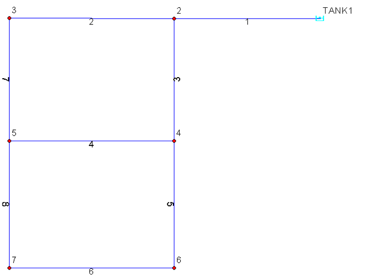
The TwoLoop project modified in this tutorial illustrates how Designer calculates pipe sizes to meet specified design criteria at the minimum cost. The TwoLoop model schematic is shown below. The model contains one treatment plant, six junction nodes, and eight pipes. All eight pipes have “dummy” diameters of 200 mm and Hazen-Williams roughness coefficients of 100. The objective is to size the existing pipes for the given network layout. A discrete diameter set of 14 values will be specified along with a minimum pressure requirement of 30 m to be maintained at each junction node.

Note:

The decision variables for this problem are the eight pipe diameters with 14 different commercially available sizes to choose from. This results in a solution space containing 14⁸ or 1.48 x 10⁹ possible designs.

During this first tutorial, you will be guided through:

Run the Designer
Creating pipe design groups
Creating design cost tables
Creating design constraints
Choosing design options
Performing a design run
Reviewing design results
Exchanging design results

Step 1: Open the TwoLoop Project

Start InfoWater Pro, and open the project TwoLoop.aprx.
Note: If you have not previously downloaded the Example files, you can do so from Quick Start Tutorial Example files.
Initialize InfoWater Pro , and then save the TwoLoop project as “Tutorial1” using the Save As command. If you wish to restart the tutorial, the original project will be available.
Click on the Apps button and choose Designer in the Apps Manager dialog box. Load the Designer from the Apps Manager.
If necessary, set the Mode to Steady State and the View to Input Data.

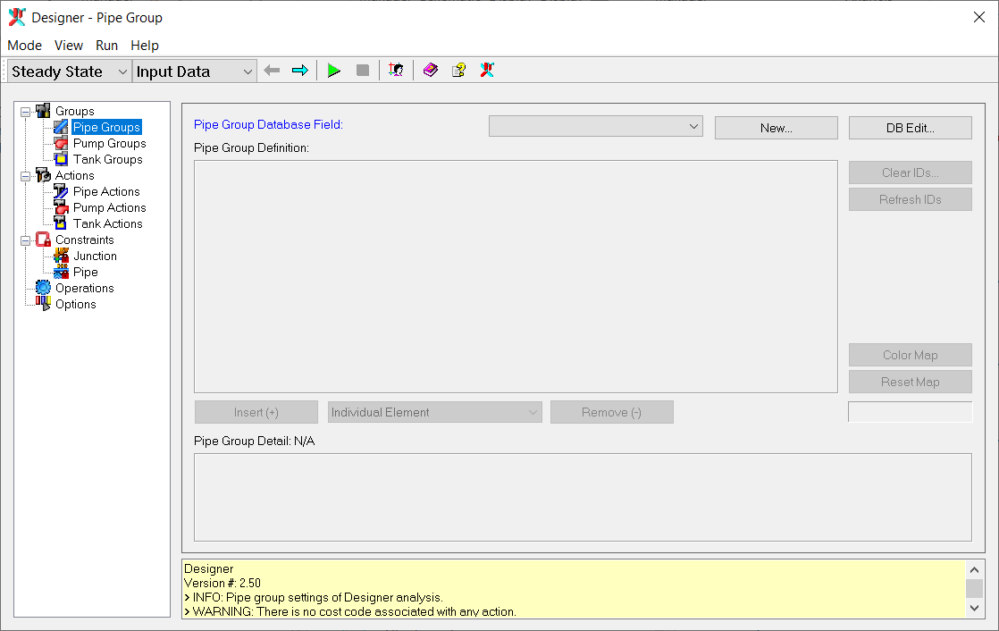
Step 2: Create Pipe Design Group

Pipe design groups must be specified before specifying other options in the designer. Pipes should be grouped together based on similar characteristics (e.g., material, age, location and diameter) and associated improvement costs. All pipes within a group will possess the same final diameter for the following three design actions: New, Parallel, and Replacement. In this example, eight pipe design groups will be created, one group for each pipe. A new database field must be added to the existing Pipe Information database table and populated with the appropriate group IDs.

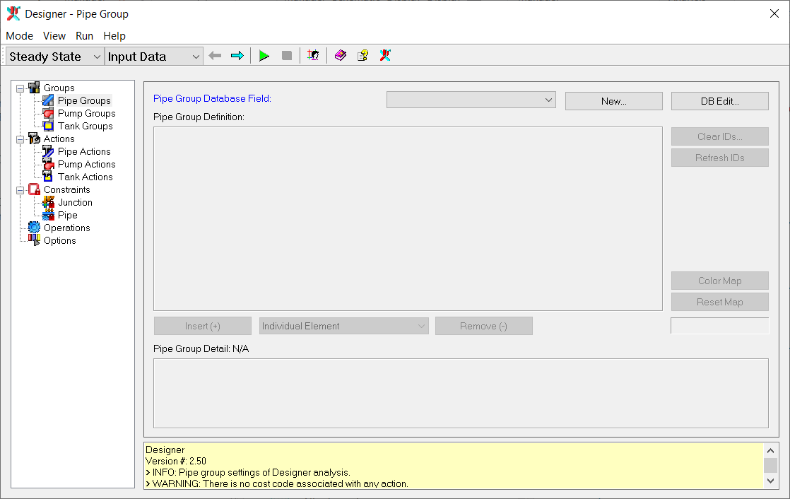
Select New and enter "PGROUP" in the Field Title, and then click OK.

The PGROUP database field now appears in the Pipe Group Database Field list.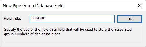
Click on the DB Edit button to open the Pipe Information table.
Enter the pipe design group ID for each pipe in the PGROUP data field. For this example, simply use the same group ID as the pipe ID. The PGROUP data field will be on the far right side of the pipe information data table.
Save the changes made to the table and then close the DB Editor.

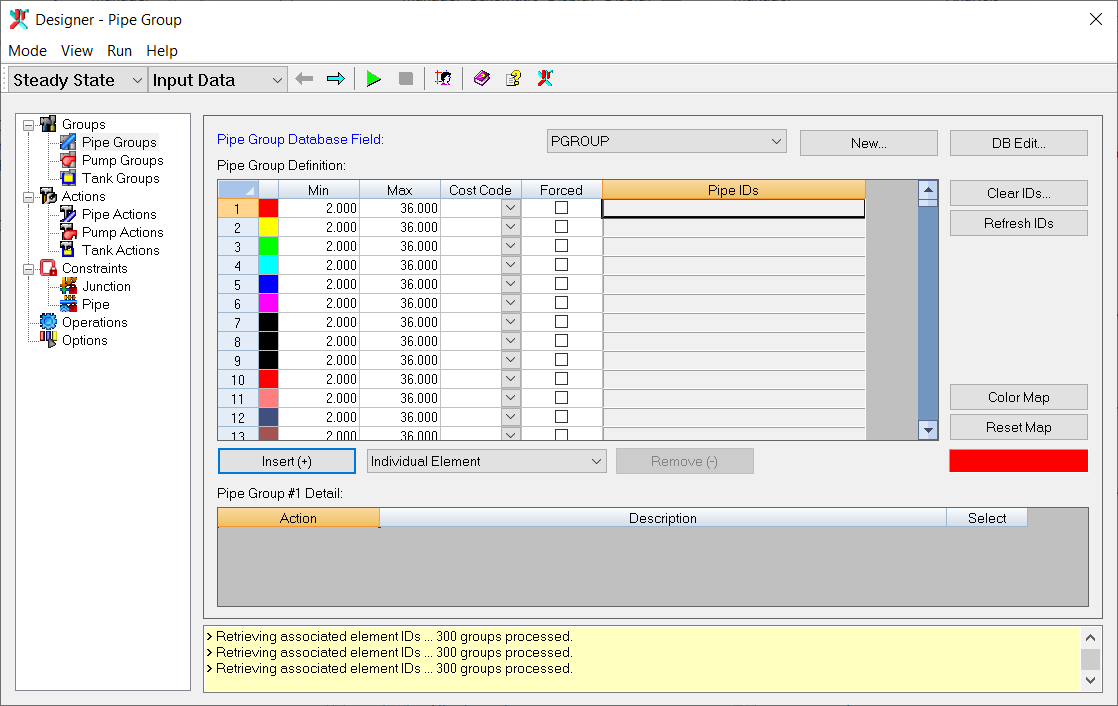
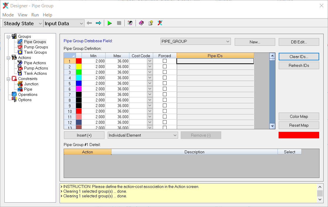
The Pipe Group Definition table is now populated.

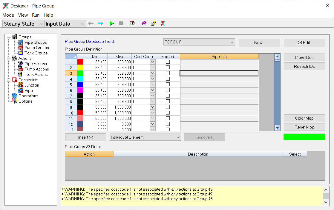
Step 3: Define Bounds for Pipe Diameters

The next step is to define the desired lower and upper bounds for the pipe diameters along with their associated cost codes and applicable actions for each of the eight design groups. Enter the following in the Pipe Group Definition table for each pipe group (1-8).

Minimum Diameter: 25.4 mm

Maximum Diameter: 609.6 mm

Cost Code: 1

Applicable Actions: NEW

Note:

Right-clicking anywhere in the table allows you to access additional commands, including copy and paste.

The Designer-Pipe Group dialog box now appears as follows:

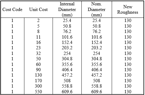
Step 4: Set Design Action Data

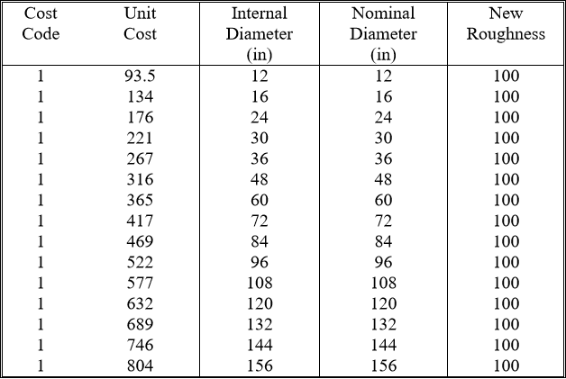
Specify the Design Action for the specified pipe groups using the Actions view. Since the entire system is new, only one Action (NEW) needs to be specified along with the set of commercially available pipe sizes to choose from and their associated costs. A total of 14 discrete pipe sizes with their cost matrix will be inputted. Enter the data as shown in the following table.

Select the Groups view and select the Action New for the eight Pipe Groups, as illustrated in the picture below for the first Pipe Group.

Step 5: Set Constraints

Using the Constraints, target minimum pressures can be defined for the entire system, for all the junction nodes within the specified domain, or for only selected key individual junction nodes. For this example, you will specify a minimum pressure of 30 meters and a maximum pressure of 150 meters to be maintained for all the junctions in the system.

Open the Domain Manager from the Designer. Add all junctions (Network Option) to the domain and close the Domain Manager. Refer to Using InfoWater Pro for more information on the Domain Manager.
Select the Constraints-Junction view and enter 30.0 in the MIN PRESSURE and 150 in the MAX PRESSURE for Domain constraints.

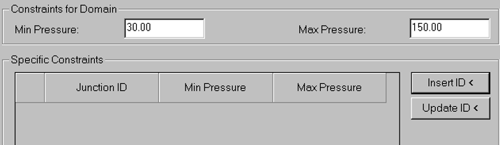
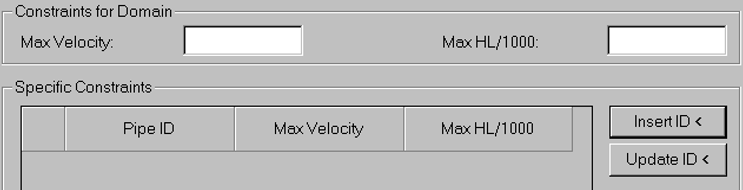
Note that if Specific Constraints for a junction were specified, they would override the Constraints for the Domain. No maximum velocities or hydraulic gradient (headloss per 1,000 unit of length) constraints for pipes will be specified for this example.

Step 6: Set Design Options

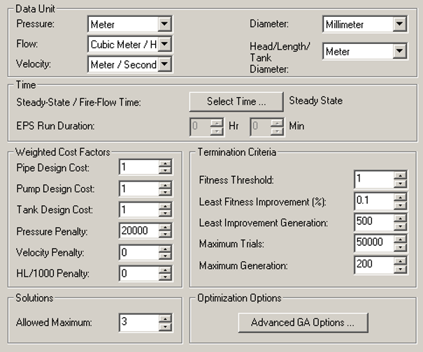
Select the Options view and specify the following GA optimization options:

Pressure Data Unit: meter
Velocity Data Unit: m/s
Pressure Penalty Cost: 20,000
Fitness Threshold (%): 1
Least Fitness Improvement (%): 0.1
Least Improvement Generation: 500
Maximum Trials: 50,000
Maximum Generations: 200
Solutions - Allowed Maximum: 3

Note:

Advanced GA Options should only be modified when you completely understands how Genetic Algorithms work.

Step 7: Run the Design Module

All required information for executing a design run is available to the Designer. Click on the Run button (or Run - > Start) to start the optimization. Click YES when prompted for Confirmation. The Simulation view appears and the statistics are updated with each trial. The figure below depicts the Simulation view after the optimization process is completed:

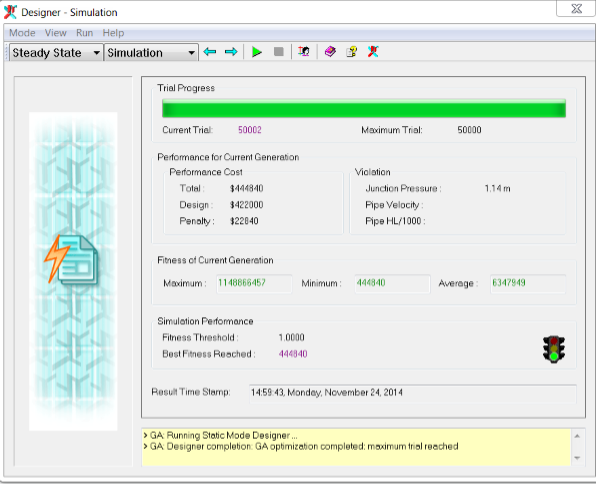
A design solution at a cost of approximately $420,000 was reached after 50,002 trials.

Note:

Since GA optimization is a stochastic search process, you may encounter local optimal solutions that differ from the global solution shown above. In case such a local solution is reached, simply rerun the design simulation to further explore the solution space to narrow the search towards the global solution.

Step 8: Review Model Results

The design results can be reviewed in the Report section of the Designer. The Report consists of five views: Summary, Pipe Group, Individual Pipe, Junction Constraint, and Pipe Constraint. Note that each view contains separate views for Pipe Group, Individual Pipe, Junction Constraint, and Pipe Constraint. SUMMARY view: Summarizes each of the three best solutions out of 50002. Three solutions were retained because the Allowed Maximum was set to 3. Note that the lowest cost solution has a greater penalty cost than the second lowest cost solution. This view is useful for looking at the total costs. PIPE GROUP view (Solution 1): This view details the pipe group results for solution 1. The determined diameters are shown, and the total length of pipe in each pipe group is shown. The total cost for each pipe group is included as well. INDIVIDUAL PIPE view (Solution 1): This view is very similar to the PIPE GROUP view, except that individual pipes are shown instead of pipe groups. This view can be used to locate pipes that may be determined to be too costly; these pipes can be placed in an alternate or new pipe group for a subsequent Designer run. JUNCTION CONSTRAINT view (Solution 1): This view contains each junction with pressure range constraints for solution 1. Pressure violations are shown in the right side columns. Minimum and maximum violations are in separate columns. PIPE CONSTRAINT view (Solution 1): This view contains each pipe with velocity or headloss violations for solution 1. These violations are shown in the right side columns.

Note:

Maximum velocity or hydraulic slope constraints were not specified for this example and therefore this view is empty.

Step 9: Change Penalty Cost and Review Results

Run another optimization with a penalty cost value of 100,000 and a maximum number of allowable trials of 100,000.

Choose Input Data from the View menu and select the Options view.
Specify a pressure penalty cost of 100,000 and a maximum trials of 100,000.
Click Run to start the optimization. Click YES when prompted for Confirmation. The figure below depicts the SIMULATION view after the optimization process is finished.
As shown in the Designer Simulation dialog box, a higher cost design solution of $446,000 was obtained after 100,002 trials.
To review the new design, click and review the results as described in Step 8.

Note:

Because of the stochastic nature of GA optimization, you may encounter optimal solutions that differ from the local solution shown below.

Step 10: Exchange Design Solution

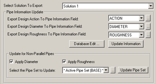
The Pipe Modeling database table can be updated with the new pipe diameters and roughness coefficients by exporting the Designer optimization results.

Choose Export from the View menu, and select SOLUTION1 to be exported.
Create new fields on the Pipe Information Table to export Designer results for Design Action, Diameter and Roughness. Click Browse on the right side of the Information Update Area and enter a name for each export field.
Check both Apply Diameter and Apply Roughness.
Choose the active pipe set to update Active Pipe Set(Base).
Click Update Information to export the Design Action, Design Diameter, and Design Roughness to the Pipe Information DB Table. (Click OK for confirmation.)
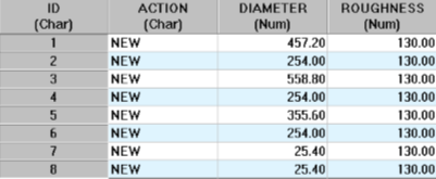
Click Database Edit to verify that the data have been exported as illustrated in the picture below.
Finally, click to update the Pipe Modeling database with pipe sizes and roughness values from the Designer results.

Note:

Exporting Data to the Information DB Table is useful for tracking changes or making a log of recommendations. The Modeling DB Table should be updated with caution; using an alternate scenario (Pipe Set) is the best option.

Example 2: NewYork System

The second example involves modifying an existing project called “NewYork”. This project should be located in the same location as the previous example. The “NewYork” project modified in this tutorial illustrates how Designer calculates parallel pipe sizes to meet the design criteria at the minimum cost. The model schematic is shown below and considers the expansion of an existing system through paralleling existing pipes. The model contains one reservoir, 19 junction nodes, and twenty-one large diameter pipes (tunnels).

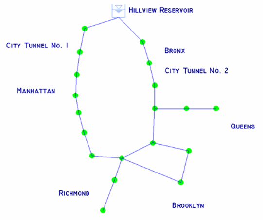
The objective is to determine which existing pipes to parallel and what size should the new parallel pipes be to supply the projected increase in demands while meeting specified pressure criteria. The new pipe diameters will be selected from 15 commercially available sizes.

Note:

For this problem, 16 decision variables including the “do nothing” option make up a solution space of 16²¹ or 1.93 x 10²⁵ possible pipe combinations.

Step 1: Open the NEWYORK Project

Start InfoWater Pro and Open the project NewYork.aprx.

Note: If you have not previously downloaded the Example files, you can do so from Quick Start Tutorial Example files.
Initialize InfoWater Pro , and then save the NewYork project as “Tutorial2” using the Save As command. If you wish to restart the tutorial, the original project will be available.
Click on the Apps button to open the Apps Manager dialog box. Load the Designer from the Apps Manager.
If necessary, set the Mode to Steady State and the View to Input Data.

Step 2: Create Pipe Design Groups

In this example, 21 pipe design groups will be created, one group for each pipe. A new database field must be added to the existing Pipe Information database table and populated with the appropriate group IDs.

Select New and enter PGROUP in the Field Title, and then click OK.

The PGROUP database field now appears in the Pipe Group Database Field list.
Click DB Edit to open the Pipe Information table.
Enter the pipe design group ID for each pipe in the PGROUP data field. For this example, simply use the same group ID as the pipe ID. The PGROUP data field will be on the far right side of the pipe information data table.
Save the changes made to the table and then close the DB Editor.

The Pipe Group Definition table is now populated.

Step 3: Define Bounds for Pipe Diameters

Define the desired minimum and maximum limits for the pipe diameters with their associated cost code and applicable actions for each of the twenty-one design groups. Enter the following in the Pipe Group Definition table for each pipe group (1-21). Minimum Diameter: 36 in

Maximum Diameter: 204 in

Cost Code: 1

Applicable Actions: PARALLEL

Note:

Right-clicking anywhere in the table allows you to access additional commands, including copy and paste.

The Designer-Pipe Group dialog box now appears as follows:

Step 4: Set Design Action Data

Specify the Design Action for the specified pipe groups using the ACTIONS view. A total of 15 pipe sizes and associated cost data will be inputted since only one Action (PARALLEL: Parallel Pipe) is specified for this example. Use the table below as a guide when entering this data.

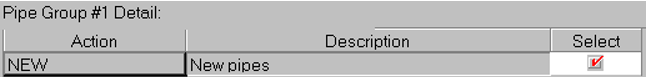
Select the GROUPS view and select the Action NEW for the Pipe Groups, as illustrated in the picture below for the first Pipe Group:

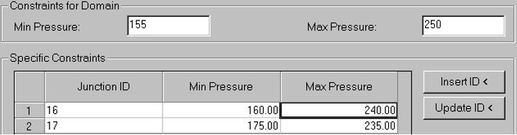
Step 5: Set Junction Constraints

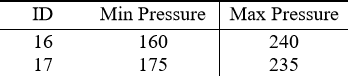
For this example, you will specify a minimum pressure of 155 ft and a maximum pressure of 250 ft to be maintained for all the junctions in the system. However, the constraint for two junctions will differ.

Open the Domain Manager from the Designer. Add all junctions (Network Option) to the domain and close the Domain Manager. Refer to Using InfoWater Pro for more information on the Domain Manager.
Select the Constraints-Junction view and enter 30.0 in the MIN PRESSURE and 150 in the MAX PRESSURE for Domain constraints.
Click Set Rows and type 2 in the dialog box. Enter the data shown in the table below.

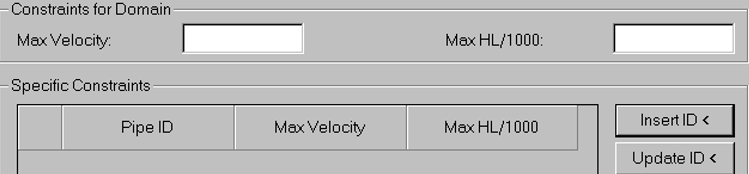
No maximum velocities or hydraulic gradient requirements for pipes will be specified for this example.

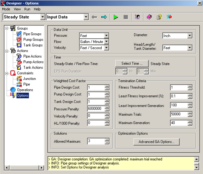
Step 6: Set Design Options

Select the Options view and specify the following GA optimization options:

Pressure Data Unit: ft
Velocity Data Unit: ft/s
Pressure Penalty Cost: 6,000,000
Fitness Threshold (%): 1
Least Fitness Improvement (%): 0.1
Least Improvement Generation: 100
Maximum Trials: 50,000
Maximum Generations: 40
Solutions – Allowed Maximum: 3

Note:

Advanced GA Options should only be modified when you completely understand how Genetic Algorithms work.

Step 7: Run the Design Module

All required information for executing a design run is available to the Designer. Click Run (or Run - > Start) to start the optimization. Click YES when prompted for Confirmation. The Simulation view appears and the statistics are updated with each trial. The figure below depicts the Simulation view after the optimization process is completed:

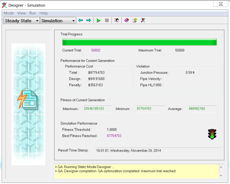
A design solution at a cost of approximately $97.75M was reached after 50,002 trials.

Note:

Step 8: View Output Report

SUMMARY view: Summarizes each of the three best solutions out of 50002. Three solutions were retained because the Allowed Maximum was set to 3. Note that the lowest cost solution has a greater penalty cost than the second lowest cost solution. This view is useful for looking at the total costs.

PIPE GROUP view (Solution 1): This view details the pipe group results for solution 1. The determined diameters are shown, and the total length of pipe in each pipe group is shown. The total cost for each pipe group is included as well.

INDIVIDUAL PIPE view (Solution 1): This view is very similar to the PIPE GROUP view, except that individual pipes are shown instead of pipe groups. This view can be used to locate pipes that may be determined to be too costly; these pipes can be placed in an alternate or new pipe group for a subsequent Designer run. JUNCTION CONSTRAINT view (Solution 1): This view contains each junction with pressure range constraints for solution 1. Pressure violations are shown in the right side columns. Minimum and maximum violations are in separate columns. PIPE CONSTRAINT view (Solution 1): This view contains each pipe with velocity or headloss violations for solution 1. These violations are shown in the right side columns.

Note:

Maximum velocity or hydraulic slope constraints were not specified for this example and therefore this view is empty.

Step 9: Exchange Design Solution

The Pipe Modeling database table can be updated with the new pipe diameters and roughness coefficients by exporting the Designer optimization results.

Choose Export from the View menu, and select SOLUTION1 to be exported.
Create new fields on the Pipe Information Table to export Designer results for Design Action, Diameter and Roughness. Click Browse on the right side of the Information Update Area and enter a name for each export field.
Check both Apply Diameter and Apply Roughness.
Choose the active pipe set to update .
Click Update Information to export the Design Action, Design Diameter, and Design Roughness to the Pipe Information DB Table. (Click OK for confirmation.)
Click Database Edit to verify that the data have been exported.
Finally, click to update the Pipe Modeling database with pipe sizes and roughness values from the Designer results.

Note:

Congratulations! You have now completed the InfoWater Pro Designer Quick-Start tutorial.