The Leakage Allocator tool provides a rough yet simple starting point to introduce background leakage into models. It is aimed at disaggregating total outflows at junctions into actual demands at junctions and pressure-dependent leakage at pipes. Most models are initially created with leakage flows combined with actual customer demands. By converting leakage from fixed amounts to pressure-dependent quantities, models can be utilized to plan and assess the effects of pressure control programs. The goal is ultimately to reduce non-revenue water volumes and extend the life expectancy of our assets.
Required information
To make use of the Leakage Allocator tool, you'll need the following:
- An identified area ("scope") where total outflows combine actual demands with leakage flows. The Leakage Allocator recognizes this area as a set of pipes, which can be:
- All the pipes in the network
- The pipes in the Domain
- The pipes in a Selection Set
- An estimate of the percentage of the combined outflow in the scope that corresponds to leakage.
For reference, the 2021 Report Card for America's Infrastructure estimates that at least 15% of extracted water for drinking supply is lost to leakage in the United States.
- A "reference" model (scenario) that roughly represents the typical dynamic behavior of your system, with outflow values that account for both actual demands and leakage flows.
- A rough estimate of the average degree of rigidity of leaks in the pipes within the scope. This is recognized as a percentage, with 0% corresponding to fully flexible leaks and 100% corresponding to fully rigid leaks (fixed-orifice-area behavior).
Optional additional information
This additional information for individual pipes can be used to increase the accuracy of the estimates for their leakage parameter:
- The degree of rigidity of leaks (0% - 100%)
- Average historic pressure
- Year of installation or repair (to compute age)
- Other custom values that relate to overall leakage likelihood
Allocating leakage
Once you've gathered the required information, follow these steps to allocate leakage:
- Activate the scenario that represents the reference network conditions.
- Define the scope.
- Run the reference standard extended period simulation. The Allocator uses the currently active scenario and output as the reference simulation.
- Optionally, create and fill custom fields in the Pipe Information DB table for individual pipe age, rigidity, average historic pressure, or other custom values.
- Open the Leakage Allocator tool from the Allocator group on the ribbon.

- Fill in the input parameters in the dialog:
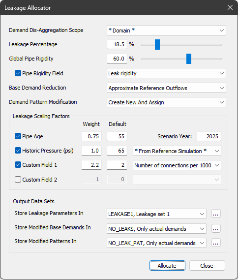
- Demand Dis-Aggregation Scope: The set containing the pipes to assign leakage to. Pipes not connected to junctions are ignored. The scope can be the entire network, the pipes in the domain, or the pipes in a selection set. Junctions connected to pipes in the scope are considered part of the scope.
- Leakage Percentage (%): The percentage of the total outflow from the junctions in the scope, during the reference simulation, to be converted to leakage.
- Global Pipe Rigidity (%): Determines the ratio of fixed and variable leakage area (see the FAVAD leakage paradigm) to be assigned to all the pipes in the scope. The ratio is evaluated at the average pressure for each pipe. With 0%, the entire leakage area is set as variable; with 100% the entire leakage area is set as fixed.
-
Pipe Rigidity Field: (Optional) Select a numerical (integer or floating point) field from the Pipe Information DB table to override the global pipe rigidity assignment for individual pipes. Values in the field should be from 0 to 100 (not 0.0 to 1.0).
-
Base Demand Reduction : Determines how base demands are reduced to make room for leakage.
-
Do Not Modify: No change to base demand values. Use this if the current total outflows in the model do not contain any leakage (only actual demands).
-
Reduce Uniform Percentage: All base demand values in the scope are reduced by the same percentage (equal to the Leakage Percentage).
-
Approximate Reference Outflows: Base demand reductions are reduced with the aim of matching the total outflow of the reference simulation once leakage is added. That is, base demand reductions are higher at junctions connected to pipes with higher leakage.
-
-
Demand Pattern Modification: Determines how to modify demand patterns to remove the contribution of leakage.
-
Do Not Modify: No change to pattern values.
-
Modify Existing Patterns: Changes are made to the patterns currently assigned to the junctions in the scope.
Warning: Outflows will also change for junctions outside the scope that use the same patterns. -
Create New And Assign: Patterns currently assigned to the junctions in the scope are copied (their name will have the suffix "_NOLEAK"), modified, and then assigned to those junctions. There is no modification to the original patterns or to their assignment to junctions outside the scope.
-
-
Leakage Scaling Factors: Select the values used to distribute leakage among pipes. The total leakage is distributed proportionately to the pipes in the scope taking into account their "leakage scores". The score depends on the length of the pipe and on the weighted sum of all its values for the selected factors. Each factor is normalized by the average value of all pipes in the scope. The Weight value assigns relative importance to each factor, while the Default value is applied to pipes with no individual value available (e.g., empty field on the table). At least one factor should be selected. Both weights and default values must be larger than zero. Please refer to the AWWA's M36 Manual for an example of the weighting of factors that affect background leakage.
-
Pipe Age: Computed using the "Year of Installation" field in the Pipe Information DB table and the Scenario Year entered.
-
Historic Pressure: Taken either from the reference simulation or from a custom numerical field in the Pipe Information DB table. Remember, the reference simulation consists of the currently active scenario and output.
-
Custom Fields: Taken from a custom numerical field in the Pipe Information DB table. Can be used, for example, to account for the number of service connections per 1000 units of length or for a custom asset-based deterioration score.
-
-
Output Data Sets: Select the data sets to store the modified model parameters in. The active set is selected as default. Click on the More button (…) to create a new set.
Warning: The current contents of the selected sets will be modified. Please do not select the active data sets if you want to maintain the data of the reference scenario unmodified.-
Store Leakage Parameters In: The leakage set in which to store the resulting leakage pipe parameters.
-
Store Modified Base Demands In: The demand set in which to store the reduced base demand values (if applicable).
-
Store Modified Patterns in: The pattern set in which to store the modified demand patterns (if applicable).
-
- Run the leakage allocation by clicking on the Allocate button.
- If the allocation is successful, click OK to return. If an error occurs, address the specific problem displayed.
- Create and activate a scenario with leakage:
- If the active output data sets were selected for the allocation, skip this step.
- If a scenario using the target data sets was created before running the allocation, activate that scenario.
- Otherwise, create a new scenario based on the reference one, and assign to it the modified data sets that were chosen for the allocation.
- Run the simulation with leakage and inspect the results.
- (Optional) Further refine the estimates for the leakage, the base demand reductions, and the demand patterns.
Leakage allocation algorithm
The goal of the leakage allocation algorithm is to convert a portion of the total outflow into leakage without significant changes to the model's behavior. The total outflow volume is aggregated from junctions at the ends of pipes within the scope and throughout the duration of the reference simulation. The algorithm assigns leakage values to the pipes in the scope so that the total leakage volume is equal to the target percentage of the total outflow volume in the reference simulation. The algorithm can also shrink the base demand values and alter the demand patterns in the scope junctions, with the reductions corresponding to the newly assigned leakage. The remaining demand values therefore represent actual demand.
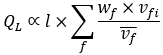
In general, the leakage parameters per unit length assigned to pipes are not the same, as they are computed so that the total target leakage volume is distributed among all pipes in the scope depending on their leakage scores. The following equation illustrates how the leakage (QL) at a pipe
i in the scope is proportional to the pipe's length (l) and a linear combination of factors
f with weight
wf and a normalized value at pipe
i of
 (
( is the average value for factor
f along all pipes):
is the average value for factor
f along all pipes):
Once the desired leakage flow at each pipe is assigned, the actual leakage parameters are computed considering the changes in pressure (p) throughout the reference simulation and applying Torricelli's law ( ).
).
If the option to Approximate Reference Outflows is chosen for the Base Demand Reduction, reductions are distributed based on the amount of leakage in adjacent pipes. The reductions are proportional in all the demand categories for a single junction, except for negative demands, which are left unmodified. When target reductions exceed the total outflow at junctions, the remaining reductions are similarly distributed among junctions with remaining capacity. Given that there are multiple aspects to be considered simultaneously, it is normal that the resulting leakage percentage does not exactly match the requested value, and that the reduced base demands do not exactly compensate for the total leakage volume. Even larger discrepancies should be expected if the option Do Not Modify is chosen for the base demands.
The modified model would ideally behave as similarly as possible to the reference model, in terms of both mass and energy balance. If demand patterns are not modified, typically the total outflow will be overestimated at night, when leakage is highest, and underestimated during peak demand periods. Conversely, pressure will be underestimated at night and overestimated during peak demand.
When patterns are modified, the algorithm computes, for each pattern and for each time step, the modification that would result in the smallest average departure from the outflow time series over all junctions in the scope. This average is weighted based on the amount of demand at each junction that corresponds to a pattern. Note that, since patterns are usually shared by junctions with different conditions and leakage values, this averaging method does not lead to a perfect match in the output time series for most junctions.