Diagrams (advanced analyses)

The option defines and displays diagrams for cases of non-linear, time history, and PushOver analyses. Diagrams let you display any result values (such as, displacements, internal forces, and stresses) collected in successive steps/increments of non-linear and PushOver analyses or in successive time increments for time history analysis. Results can be displayed as a function of successive increments (iteration steps or time steps) and as a function of other quantities.

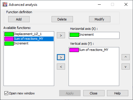
Note: You can display on a diagram 'n' different quantities (shown on the vertical Y axis) as a function of only one quantity provided on the horizontal X axis.

After you click Results menu > Advanced > Diagrams, the following dialog displays. (In the menu of the non-linear analysis table this is the option: Results > Non-linearity > Plasticity/Diagrams; whereas, in the menu of the pushover analysis table this is the option: Results > Advanced > Pushover Analysis - Diagrams).

A load case for which the defined diagrams are to be displayed can be selected from the Cases selection list in the top toolbar of Robot. Diagrams can be displayed for a single case or for several selected cases.

If different types of load cases are selected (the selection includes cases of non-linear, time history as well as PushOver analyses), diagrams can be displayed only for one analysis type. (The top priority is given to non-linear and PushOver analyses cases.)

The dialog has the following options:

Function definition field:
- Add - Opens the dialog to define a new function.
- Modify - Opens the dialog for function definition (change of name or values of the function currently selected in the Available functions field).
- Delete - Deletes the function definition currently selected in the Available functions field.
The left side of the dialog comprises the Available functions panel where all the functions defined in the Diagram definition dialog are included. In the middle of the dialog, standard buttons are provided for transferring the contents of the panels:
- Next to the Horizontal axis (X) field:
  > - Moves a selected diagram to the field (functions that have been moved, still remain in the Available functions panel).
- Next to the Vertical axis (Y) field:
  > - Moves a selected diagram to the panel (functions that have been moved, still remain in the Available functions panel).
  
  < - Deletes a selected diagram from the right panel.
The right side of the dialog has 2 fields (panels):
- Horizontal axis (X):
  A quantity located in this panel determines the diagram horizontal axis. Note that only 1 quantity (such as, displacement, increment) can be provided in this field.
- Vertical axis (Y):
  A panel containing quantities that determine the diagram's vertical axis (you can display many diagrams in one drawing).
Open new window - When selected, a view with diagrams opens as a new window.

Note: The Apply button is available only when a complex case is active in the view, i.e. a case containing results saved for the component increments. The time history, non-linear and push-over analysis are such cases. The Apply button is not available if the common static cases are active.

For the non-linear analysis cases, only the result of the last load increment is saved as default. The diagrams will not be available for such a case. The option 'Save results after each increment' should be activated for a non-linear analysis in the Analysis/Analysis types dialog in order to save results for each increment.

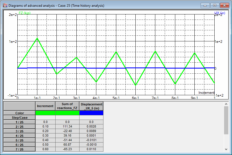
After the diagrams are defined and moved to the Horizontal axis and Vertical axis fields in the Advanced analysis dialog, clicking Apply displays a view showing the selected diagrams. After clicking Close, the Advanced analysis dialog closes. When it reopens, the diagrams defined are available.

The top of the view has the diagrams of the selected quantities provided in the same drawing. At the bottom, there is a table with a diagram description and the extreme values of the selected quantities (in the first column information about the X axis is located; whereas, the second column has information about the diagrams displayed on the Y axis). Elements displayed in the table can be set using the Table Columns option from the shortcut menu, which appears when you right-click inside the table.

The shortcut menu also includes the Diagrams - properties option displays selected information on diagrams.

Descriptions of the diagrams are turned on after selecting the Diagrams descriptions option in from the shortcut menu. A description of each diagram shows the minimum and maximum values on the diagram.

Note: If several load cases have been selected, each of the defined diagrams is displayed for successive cases (in other words, 'n' different diagrams are generated). A range on the X axis is determined by <min, max> of all the load cases; for the range on the Y axis, it is defined by <min, max> of all the load cases (corresponding to each scaling type).

Diagrams (advanced analyses)

Was this information helpful?