After a simulation is run, the graphics region updates to display the results for the analysis type in the form of a volume plot (default display). The various results types populate the Results browser folder. To see the variety of results you can view, expand the Results folder.
| Simulation Type | Result displayed |
| Static Analysis | Displays the Von Mises Stress plot |
| Modal Analysis | Displays the first frequency mode. |
To view a different result, right-click the browser node corresponding to the results you want to see and click Activate, or, double-click the result browser node. The graphics region updates to display the selected results type.
There are several display options available for interpreting the simulation results.
Volume Plots
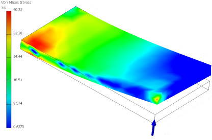
The graphics region displays a volume plot and a color bar displays the range of the variable showing in the graphics region. Color order is as follows, from high values to low values: red, orange, yellow, green, cyan, and blue.
Parametric Study Configurations
For Parametric Studies, you can move sliders in the Parametric Table to display the different configurations. If the configuration was not generated, the message “Not Available” displays in the graphics region. You can right click the parameter row and select Generate Single Configuration, or run the simulation to solve the configuration.
Smooth Plot
Smooth shading is the default plot presentation for all result types, whether Static or Modal analysis simulation. Colors blend from one to the next.
Contour Plot
The contour plot presents the colors using a strict banding method. Color separation is clearly seen.
Change the shaded display:
- In the Display panel, click the Shaded Display command to display the pull down list.
- Select from Smooth Shading, Contour Shading, and No Shading. The graphics region updates.
Mesh
At any time, you can click Mesh View to overlay the mesh on the volume plot. The Mesh View command is an On/Off display toggle once the mesh has been defined.
XY Plots
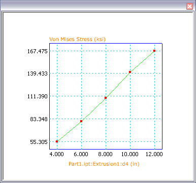
With parametric studies, you can view the results as a two-dimensional XY plot.
- In the browser, select the Results type (Von Mises Stress, Displacement, and so on) you are interested to see in a plot.
- Right-click the parameter row and click XY Plot. A window with the XY Plot is displayed over the graphics region. The window is resizable.
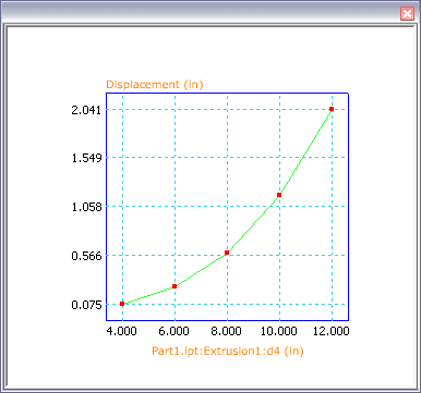
The following image is from the same simulation as the preceding image. However, the XY Plot is for Displacement results rather than Von Mises Stress.
Convergence Plots
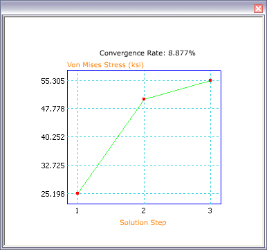
You define the convergence criteria that is used to reach a solution. You can then view the resulting convergence plot which shows the number of refinements used and the parameter values associated with each refinement.
To view an XY plot of the result convergence, you must have edited the Convergence Settings and set the Maximum Number of h Refinements to greater than zero. Right-click the Results folder node in the browser, and click Convergence Plot. The convergence criteria is set in the Convergence Settings dialog box.
- In the Prepare panel, click Convergence Settings. The dialog box displays.
- Specify the Stop Criteria percent of convergence required.
- Specify the Results type on which to converge.
- Specify any Geometric Selections
- Specify the Maximum Number of h Refinements to use.
- Specify the h Refinement Threshold.
- In the Solve panel, click Simulate. Let the simulation complete.
- In the Result panel, click Convergence Plot. The plot is displayed in a window over the graphics region.
Deformation Plots
Most often, the true geometry deformation is slight in comparison to the overall model size. In order to understand where deformation is occurring an automated exaggeration effect is provided. The Adjust Displacement Display command provides the following display options:
- Undeformed
- Actual
- Adjusted x0.5
- Adjusted x1
- Adjusted x2
- Adjusted x5
When the volume plot is displayed, select one of the display options to exaggerate the deformation.
Animate Results
You can animate the simulation results and retain the animation for your records by producing video output.
Maximum and Minimum Results
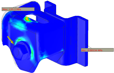
Commands for easily locating the maximum and minimum result values are located in the Display panel.
Click the Maximum Result![]() command to display an annotation at the point where this condition occurs.
command to display an annotation at the point where this condition occurs.
Click the Minimum Result![]() command to display an annotation at the point where this condition occurs.
command to display an annotation at the point where this condition occurs.
Probe Labels
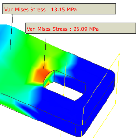
You use the Probe![]() command to identify points of interest with a label specifying the result type and value at that point. You can annotate as many points as you want. The Probe Labels
command to identify points of interest with a label specifying the result type and value at that point. You can annotate as many points as you want. The Probe Labels![]() command turns visibility on and off for those labels.
command turns visibility on and off for those labels.
Boundary Conditions
The Boundary Conditions![]() command turns on and off the display of the load indicator, which points to where the load is applied.
command turns on and off the display of the load indicator, which points to where the load is applied.