After the simulation finishes, the graphics region displays a 3D color plot, and you can see that the Result folder is populated. Now we can evaluate the results through the parametric table and the 3D and XY plots available for post processing.
Optimize model
First, we optimize the mass using the parametric table populated in previous steps. Then we look at 3D and XY plots to understand the behavior of the model under the defined boundary conditions.
The goal is to minimize the mass of the model taking into account parametric dimensions and stress constraints.
- If you previously closed the Parametric table, reopen it by clicking the Parametric Table command.
- For the Mass Design Constraint, click in the Constraint Type cell, and select Minimize from the drop-down list.
The parametric values change to show the configuration with the least mass that meets the given constraints. In this case, the original thickness value was 12 mm and the optimized value is 9 mm which in turn reduces the mass of the model.
Note the design constraint Result Value for Max Von Mises Stress. The value has a green circle preceding it. It indicates that the design constraint value is within the safety factor range.
Slide the Extrusion1 parameter value to 6. When the table updates, you will see that the design constraint Result Value is now outside the safety factor. The value is preceded by a red square indicating the design constraint value has been exceeded the safety factor. Slide the parameter value back to 9.
View and animate 3D plots
Now you can perform post-processing tasks using the Display panel commands for smooth shading, contour plots, etc. These commands are described in Help.
- In the Result panel, click Animate Results.
- In the Animate dialog box, click the Play
 command. The Von Mises Stress plot colors change to reflect the application of the load. To view the deformation changes, stop the animation, select Adjusted x1 from the Adjust Displacement Display
 , drop-down list and restart the animation.
For post-processing of results, double-click the result in the browser to display the result in the graphics region. Then, select the Display command you want to use.
View XY graphs
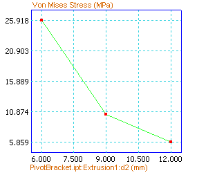
XY Charts show a result component over the range of a parameter.
To view an XY plot, right-click over the parameter row in the Parametric Table and choose XY Plot.

In this case, the above XY plot displays Stress results versus parametric configurations.