For problems with very few degrees of freedom, the determinant could be evaluated explicitly, giving a polynomial of order N in  ( N is the number of unconstrained degrees of freedom).
There will be N real roots, and  is simply equal to the smallest (in magnitude) of these roots. Back substitution of into the buckling equations will give the critical buckling displacement mode. This mode is defined as an arbitrarily scaled set of displacements corresponding to the change of configuration that occurs during buckling. Therefore, if we wish to view the postbuckled configuration of the structure, it is necessary to superimpose the critical displacement mode associated with , on the undeformed configuration of the structure.
For structures having many degrees of freedom, the determinant expansion followed by root extraction method becomes unworkable. To utilize a more general solution algorithm, it is necessary to identify the buckling equations with a generalized eigen-problem. Associated with this eigen-problem there are N real eigenpairs  ,
,  , where i = 1,...N , and and are, respectively, the ith eigenvalue and eigenvector representing the ith critical load factor and buckling displacement modes. Powerful, general purpose, methods are available to solve generalized eigen-problems. The method used is called the subspace iteration method [1].
Using the subspace iteration method, we can find a series of say n eigenpairs arranged in order of increasing magnitude of , that is, from which it follows that =
 and
and  = .
= .
The number of eigenvalues to find is a parameter which you can specify during a Warp or Stress analysis. Note however that the computational effort involved increases markedly as the number of eigenpair solutions required increases. Moreover, in a buckling problem, one is normally interested only in the "real" critical state rather than in hypothetical higher-order modes. While it is not uncommon, under increasing load, for a structure to change (usually via bifurcation) from the first critical mode into another higher-order mode, it is quite wrong (and dangerous) to assume that the load level and buckled shape corresponding to the latter mode are meaningfully related to the first mode predicted. The reason is that during the transition from the lower to the higher buckling mode, the configuration of the structure is likely to undergo significant change, thus creating an obvious conflict with the basic assumptions of the buckling analysis.
Sign of Predicted Eigenvalues
Note that there is no restriction on the value of , both positive and negative values are admissible. Thus, for example, if  is selected so that it creates a tensile stress field in a flat plate, then will be negative. On the other hand, reversing the direction of , so the stress state is compressive, will lead to a positive value of . By definition, however, both values will have exactly the same magnitude. If the reference loading is reversible, then in practice it suffices to find the first eigenpair alone (this follows because we know that when is negative, reversing the direction of will simply reverse the sign of ). A difficulty arises, however, when we consider an irreversible load system. In this case buckling will correspond to the lowest positive eigenvalue, and since it is impossible to tell in advance how many negative eigenvalues there are, we must either proceed on a trial-and-error basis, or do a single analysis in which at least two eigenpairs are requested. Experience to date with irreversible load systems (for example, shrinkage strains acting on a plastic component) indicates that the solution of the first two eigenpairs is usually sufficient (that is the values are either both positive, or one is negative and one is positive).
Sturm Sequence Check
Using the subspace iteration method, it is occasionally possible to skip one or more eigenvalues, as one or more eigenvalues that actually exist may be missing from the values that are predicted. For this reason, a technique called the Sturm sequence check, is used to check for missing eigenvalues. Unfortunately, the check is not valid if any of the n eigenvalues are negative.
Validity of Buckling Result
When conducting a buckling analysis, it is important to bear in mind the limiting nature of the initial assumptions. If there is substantial change in shape before buckling, then the results will become unreliable because the method is being applied outside its range of validity. Usually, this means that will be over-estimated, but this is not always the case. If there is reason to believe that the prebuckling displacements of the structure are not small, then the buckling analysis should always be followed by a full large deflection analysis.
Types of Buckling
-
Limit point.
-
Bifurcation.
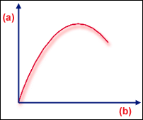
Limit point
.(a) load, (b) deflection
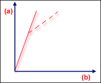
Bifurcation of Perfect Structure
.(a) load, (b) deflection
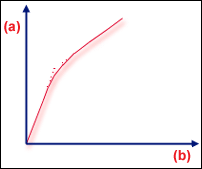
Bifurcation of Real Structure
.(a) load, (b) deflection
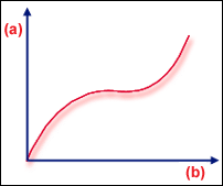
Softening then stiffening
.(a) load, (b) deflection
A Limit point, loosely speaking, is a state where the component can accept no more load without a major change of shape (GUID-065E2D92-2B4E-4450-8CF3-767A371CCE17.htm#FIG_8E8E00D024E74D96B307638F66391293). This typically occurs in dome-shape components, where a central load may cause the dome to "snap-through". More generally, we expect buckling to be of the limit point type when there is significant geometric non-linearity before the buckling point. In the dome example, the component needs to become fairly flat before the stiffness matrix determinant becomes zero. After the "snap-through" (which may be gentle or severe), the component can accept more load, but generally components must be designed so that expected loads do not reach the limit point.
A bifurcation is a "branching" point where two possible equilibrium states lie close together. If you think of a perfectly symmetrical flat plate, then the response of the plate to an in-plane compressive load is simply linear. However, once the load exceeds a critical value the equilibrium becomes unstable; like a ball at the top of a hill-which way will it roll down? So a real flat plate will buckle at that critical load level. Thus we have two possible equilibrium paths and we call their intersection a "bifurcation point" (GUID-065E2D92-2B4E-4450-8CF3-767A371CCE17.htm#FIG_5D265CECEBA9443783273002C74E6C0D).
Both these types of buckling can appear in warpage or thermal loading problems, although bifurcation is more common. In the flat plate example, imperfections in the plate cause a blurring of the sharp change of stiffness at the Bifurcation point (GUID-065E2D92-2B4E-4450-8CF3-767A371CCE17.htm#FIG_4E53D06197A342F49024EDB4A75BF2C0). Another common response is "softening followed by stiffening" (GUID-065E2D92-2B4E-4450-8CF3-767A371CCE17.htm#FIG_8A331E70626C4AE6AEADA8D8552CFE99). In this case, the determinant of  falls to some small value, but not zero.
Buckling analysis of cases like GUID-065E2D92-2B4E-4450-8CF3-767A371CCE17.htm#FIG_5D265CECEBA9443783273002C74E6C0D and GUID-065E2D92-2B4E-4450-8CF3-767A371CCE17.htm#FIG_4E53D06197A342F49024EDB4A75BF2C0 usually give a good indication of where the bifurcation is. Analysis of cases like GUID-065E2D92-2B4E-4450-8CF3-767A371CCE17.htm#FIG_8E8E00D024E74D96B307638F66391293 tend to overpredict the limit point. In problems like GUID-065E2D92-2B4E-4450-8CF3-767A371CCE17.htm#FIG_8A331E70626C4AE6AEADA8D8552CFE99, there is no clear-cut buckling load, however the buckling analysis will often indicate where the non-linearity starts to become severe.
References
1. Bathe, K.J., Finite Element Procedures in Engineering Analysis, Prentice-Hall, Englewood Cliffs, New Jersey, 1982, pp. 666-696.