Small deflection Stress analysis (Concept)

Small deflection analysis is the most common type of analysis and is the basis of both large deflection and buckling analysis. A thorough understanding of small deflection analysis is an important prerequisite for understanding the other analysis types.

Small deflection analysis is also frequently called linear analysis.

Assumptions

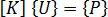
Small deflection analysis is based on the assumption that the displacements and corresponding stresses and strains, resulting from the application of loads to a flexible body, are a linear function of the magnitude of such loads.

To achieve this linearity, we must assume that the material from which the body is made is elastic and that the displacement gradients are small enough everywhere to neglect the effects of the associated changes in geometry. In other words, we must assume that the body behaves as if it is both materially and geometrically linear. That is, the resulting change in geometry does not significantly alter the stiffness of the structure. Under these conditions, the governing equilibrium equations take the familiar form:

where:

is the assembled stiffness matrix of the idealized structure,
is the unknown nodal displacement vector, and
is the vector of equivalent nodal forces.

Constitutive Model

Within the restriction of a linear elastic material (a material which obeys Hooke's law), it is nevertheless possible to include both homogeneous and non-homogeneous materials. In the present case, for shell elements (LMT3, LBT3), we will however assume that the material is homogeneous with respect to the thickness direction. With this restriction, the material properties can vary from one point in the structure to another, but at each point there will be two orthogonal directions with respect to which the elastic moduli take on principal (that is, maximum and minimum) values. These directions are called directions of orthotropy and the associated material model is called orthotropic.

Two alternative elastic material models are available. The first is an isotropic model (material is non-directed and homogeneous). The second is a special case of the orthotropic model described above, in which any point-to-point variation in the values of the principal moduli is ignored (material is multi-directed but homogeneous). The latter model is applicable to molded plastics since it accounts for the molecular orientation effect that occurs during the molding process.

Boundary Conditions

Prior to the application of boundary conditions, the equilibrium equations will be singular, that is, the stiffness matrix will not be positive-definite and its inverse cannot be found. However, the stiffness can be rendered positive-definite by application of a suitable set of displacement boundary conditions. The resulting "reduced" set of equations will be determinate (that is will be positive-definite) provided all possible rigid-body displacement modes have been removed. In practice, provided the finite element model is free from internal releases (for example pins) and the elements themselves do not contain any spurious zero-energy modes, then an admissible set of displacement constraints is any set that provides a finite (greater than zero) resistance to each of the six possible rigid-body movements of the structure.

To categorize available forms of displacement constraint, it is useful to imagine that the movements corresponding to each degree of freedom at a constrained node are resisted by external (that is linked to ground) springs. The three most common forms of displacement boundary condition are then:

Rigid (displacement is zero, spring stiffness is infinite).
Semi-rigid (displacement non-zero, spring stiffness finite).
Prescribed (displacement takes a non-zero prescribed value, no spring).

There are two alternative ways of dealing with a rigid constraint. The first method is simply to remove the corresponding equation from the overall set. The second method is to replace the requisite leading diagonal coefficient of

, namely

, by a coefficient, say

, that is large enough to uncouple the constraint equation from the remaining set. At the same time, the i^th component of the force vector

should be set to zero. The latter technique is easily extended to the prescribed displacement case by simply setting the i^th component of

to:

where is the required displacement. The advantage of retaining the full (original) equation set is that the information needed to calculate reactions at constrained nodes is directly available during the back-substitution phase.

Applied Loads

The generalized load term is called an equivalent load vector because it accounts for the effects of distributed loads such as pressures, tractions, body forces, initial strains or initial stresses, as well as concentrated loads applied directly to the nodes. In the former case, a system of nodal forces can always be found that is in equilibrium with the specified distributed loading. For simple elements, these forces will be statically equivalent to the applied load (that is they may be found from statical equilibrium conditions alone), but in other cases a detailed knowledge of the element formulation is required to determine their values. The contribution of any distributed loads to is evaluated automatically by the analysis.

Small Deflection Analysis Solution

Once the boundary conditions and applied loads are known, the nodal displacements are found from:

In practice, it is unnecessary and inefficient to invert when solving the above equation. Instead the above equations are solved by Gaussian elimination.

Banded Stiffness Matrix

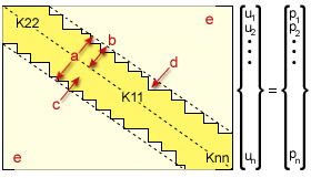
(a) Bandwidth, (b) Semi Bandwidth, (c) Profile, (d) Skyline, (e) All Zeros Outside Band.

The stiffness matrix , has three properties that make Gaussian elimination very efficient:

The matrix is symmetric (that is, the entries on one side of the main diagonal are "mirror images" of those on the other. The main diagonal is the imaginary line from the top left to the bottom right entries.
Most terms in the matrix are zero.
In the matrix all the non-zero terms lie within a narrow band centered about the main diagonal.

GUID-1B128FF9-2E3A-4170-8984-618E66FA4675.htm#FIG_CC0126A4A95B49269FA4E00BEA936191 illustrates the appearance of the stiffness matrix. The boundary between the (mostly) non-zero terms and the all zero terms is termed the skyline. The set of coefficients between the main diagonal and the skyline is referred to as the profile. Since the matrix is banded and sparse, processing time is decreased by only performing elimination within the profile. The symmetry of further reduces the amount of calculation since the part of yet to be eliminated remains symmetrical any stage in the elimination, and so calculation of the known symmetric terms is not required.

For maximum efficiency, the number of coefficients within the profile is first minimized using a nodal re-numbering scheme (the re-numbering is entirely transparent to the user). The bandwidth optimization algorithm adopted is due to Gibbs, Pool and Stockmeyer [1].

Often, the number of equations involved in an analysis is too large to fit all the coefficients in virtual memory (for historical reasons we say "core" for virtual memory). To solve such large systems of equations, an "out-of-core" solver is used in which the full matrix is kept on secondary storage (usually a hard disk drive). Thus, if necessary, the full matrix is divided into blocks and the Gaussian elimination carried out with only two blocks resident in "core" at any one time (one block is being reduced while the second block contains the coupling coefficients). The minimum block size is equal to the maximum semi-bandwidth of . The maximum block size is machine dependent, but a value that is appropriate to achieving optimum efficiency will automatically be assigned by the program (the highest efficiency usually coincides with the use of a minimum number of large blocks).

Multiple Load Cases

Stress and Warp analysis give the option to specify more than one load case for the analysis, that is different shrinkage strains or external load cases. These multiple load cases can be solved very efficiently because the structure stiffness matrix is formulated once and then used to determine the displacements for each load case. Each load case appears as a row in the Job Progress table written to the result file of the analysis.

Analysis Output

Once the displacement field is known, the strain-displacement and stress-strain relations of each element are used to determine strain and stress levels at various positions within the element. In FENAS, these positions will automatically be selected so that they coincide with the numerical integration stations used when integrating over the element volume to find the element stiffness matrix. The use of numerical quadrature stations as stress/strain recovery points is optimum or near-optimum.

Apart from echoing the input data, the analysis output file includes reactions at constrained and initially displaced nodes, nodal displacements and element stresses.

By definition, all these quantities are a linear function of the applied loading-thus, for example, if the loading is halved, the displacements, and stresses will also be halved. This allows you the freedom to choose any nominal intensity of loading without affecting the qualitative validity of the results. Care must however be exercised when extending this concept to include the influence of material constants. If the structure is externally loaded, the strains and displacements will be inversely proportional to the material constants (for an orthotropic material, to maintain proportionality it will be necessary to hold the ratio of the material moduli constant), but stresses will remain constant. On the other hand, if an unconstrained structure is subject to "internal" loading, such as that caused by temperature changes or free shrinkage, then the stresses will be proportional to the material's mechanical properties. The displacements will remain constant. Finally, for a problem involving both internal and external loading, both displacements and stresses become dependent on the material moduli.

Results interpretation

The recommended procedure to use once the first small deflection solution has been obtained is to check that the results are sensible. The best way to do this is by looking in detail at the displacement field. This is easily done using the graphical post-processing facilities.

The questions to ask are:

Does the pattern look sensible?
Are the magnitudes roughly what you expect?
Are any expected symmetries being reproduced? In general, such symmetries can only be reproduced if the geometry, loading and boundary conditions are all symmetric. Note that if the finite element mesh is itself non-symmetric, then any expected symmetry in the results will rarely be reproduced exactly.

Once you are satisfied that a consistent displacement field has been obtained and that the average stress levels make sense in relation to specified material data and other parameters, it will be necessary to decide whether or not a second analysis using a finer mesh should be undertaken. The reason why, in general, the solution for two different mesh densities is required is simply that the finite element method always leads to an approximation to exact or fully converged solutions. By implication, an objective measure of accuracy can only be arrived at by looking at the changes that occur in the results for the two meshes.

To expand on this important point, in a stress analysis suppose you wish to achieve an accuracy of at least 95% in the predicted peak level of von-Mises stress, and have obtained two values of this stress corresponding to the two different meshes. If the change in stress for the two meshes is less than 5% then, providing convergence from this point is assumed to be monotonic (which will generally be the case if the target accuracy lies roughly in the range 95%-100%), then the target accuracy has been exceeded for the finer mesh. On the other hand, if the change is greater than 5%, then further finer meshes must be used and the process repeated until the target is achieved. Note that when the solutions for only two meshes are known and the finer mesh passes the test, it is impossible to say whether or not the coarser mesh would also pass (to answer this question it is necessary to analyze a third mesh that is coarser than either of the original pair).

Against this background it should be clear that there is really only one situation in which a second finer mesh solution might be deemed unnecessary. This is when you have sufficient experience based on previous finite element analyses of similar problems to be confident that the mesh you used is adequate from the point of view of the precision required.

Relevance of Small Deflection Analysis

There are three main reasons why small deflection (as opposed to large deflection) analysis is a valuable tool in its own right:

Small deflection analysis offers the fastest and most effective way in which useful and consistent information about the mechanical behavior of a structure can be obtained.
Small deflection analysis provides an excellent tool for building up an understanding of and insight into a wide range of "structural mechanics" problems. Moreover, until some understanding of the small deflection response has been gained, you will have no chance at all of understanding the corresponding large deflection response.
Small deflection analysis provides the only cost-effective way in which to decide on mesh density and mesh distribution. Because non-linear analysis can be viewed as a series of linearized steps each of which is governed by a different set of starting conditions, it is generally accepted that accuracy checks made on the basis of a small deflection convergence study are approximately valid in the large deflection range as well.

References

1. Gibbs, N.E., Poole, W.G., and Stockmeyer, P.K., "An algorithm for reducing the bandwidth and profile of a sparse matrix", S.I.A.M. Journal on Numerical Analysis, Vol. 13, No. 2, 1976, pp. 236-250.