Large deflection Stress analysis

In practice, most structures will exhibit a linear or approximately linear response only over a restricted range of load intensities. At higher loads the stiffness of the structure can alter significantly, leading to a non-linear response.

As a simple, but nevertheless realistic illustration of non-linearity, consider a slender column of length L subject to a horizontal force H and a downward vertical force V at the top (bottom is clamped, top is free). Ignoring the small downward movement of the tip, the primary effect of such a load system will be to deflect the top of the column laterally by an amount, say u. If we now consider the structure and loads in this displaced configuration, it is immediately apparent that the bending moment M at the column base is now:

M = HL+Vu

The fact that M is not simply a function of the external loads but depends on u as well, shows us immediately that the problem is non-linear. Evidently, the effect of the vertical load acting on the bent column will be to further increase the lateral displacement, so that direct solution of the problem is not possible. We can however get close to the true solution by dividing the applied loads H and V into small increments and progressively building up the load to the required level.

As each new increment of load is applied, we can calculate the lateral stiffness of the column tip in its current displaced configuration and then solve to find the corresponding increment in u using

where:

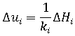
• i is the increment number and
• k_i is the current lateral stiffness of the column tip.

If we now draw a load-deflection graph taking H_ias the load and u_i as the displacement, a curve will be obtained whose slope at the origin is equal to the initial linear stiffness, k₀, of the tip, that is,

where E is the elastic modulus and II is the second moment of area. As the load increases, the slope of the load-deflection graph decreases. This is referred to as a softening response (GUID-319C546E-931F-41D8-805E-130A648F79E8.htm#FIG_77EDBD33E8704945BC1FCC614233D5EE, left). Usually, if the loading creates compressive stress (as in this example), the non-linear response will be of the softening type, whereas, if it creates tensile stress (for example, a laterally loaded beam whose ends are not free to move inwards), a stiffening response (GUID-319C546E-931F-41D8-805E-130A648F79E8.htm#FIG_77EDBD33E8704945BC1FCC614233D5EE, right) will generally ensue.

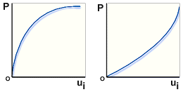
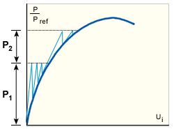
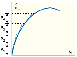
Load-Displacement Plots for Non-linear Response

.

Left softening response, Right stiffening response, P Nonlinear Load, u_i Displacement Plots

In the above example, we used an approximate method of following a non-linear load-deflection path-in this method, the true or exact response could only be found by taking infinitely small steps. To understand the basis of a more exact model of non-linear response, it is necessary to recognize that the structure must be in equilibrium at each point on a true load-deflection path. In fact, what is really happening is that as the load is increased, the structure takes on successive configurations that are uniquely determined by equilibrium alone. For this reason, any curve drawn in load-displacement space is more correctly referred to as an equilibrium path. In a structure with many degrees of freedom, the various coefficients of the stiffness matrix will vary at differing rates as the intensity of load varies. Consequently, the equilibrium paths obtained by plotting different displacement components against the applied load may look quite different. The seemingly arbitrary selection of suitable components to plot is forced on us because the full (generalized) non-linear response actually leads to a surface in an (N+1) -dimensional load-displacement space (here, N is the number of free displacement degrees of freedom of the structure).

Equilibrium Equations

The basis of the large deflection analysis model used by the analysis is a set of incremental equilibrium equations spanning the full set of nodal degrees of freedom of the structure. These equations can be written:

or

where:

• is the linear stiffness matrix for the current configuration.
• is the initial stress or geometric stiffness matrix for the current configuration.
• is the vector of incremental nodal displacement.
• is the vector of nodal forces equivalent to the current level of externally applied loads.
• is the vector of nodal forces equivalent to the internal stress field.
• is the tangent stiffness matrix for the current configuration.
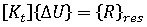
• is the vector of residual (unbalanced) nodal forces in the current configuration.

These equations are non-linear and cannot be solved directly. Instead we can employ any of the classical predictor-corrector iterative techniques (for example, Newton-Raphson or quasi-Newton) where the left-hand side is used as the predictor and the right-hand side as the corrector. During a normal (successful) set of iterative cycles, the configuration of the structure will converge towards the true equilibrium configuration and simultaneously the residual out-of-balance forces, , will become arbitrarily small. In practice, the iterations are terminated when a target accuracy (defined by the program or by you) is achieved. Note that during equilibrium iterations the load level is normally held constant.

Solution Methods

For each solution step, the non-linear equilibrium equations are linearized around the current configuration of the structure. The associated linearization errors result in residual unbalanced forces at each node of the finite element mesh. Iterations of the Newton-Raphson (NR) type are therefore required to reduce these unbalanced forces to acceptably small values. This process is called equilibrium iteration. The full Newton-Raphson algorithm involves reformation and factorization of the global stiffness matrix at the beginning of each iterative cycle. Although this generally results in optimum convergence rates, it is nevertheless very costly. To alleviate this problem, a number of more cost-effective strategies can be used. A total of six such strategies (including NR) are available in the analysis. They are:

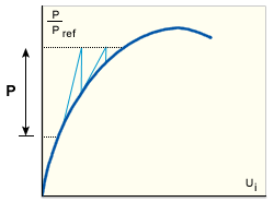
KSTRA=0: Initial stiffness method

In this very cheap but rather crude method, the initial linear elastic stiffness is used for all loading increments and each iterative cycle within an increment (GUID-319C546E-931F-41D8-805E-130A648F79E8.htm#FIG_4CA25ED1D4EB4624A4923EA6BD146F6C). Because the prediction of displacement increments is always based on linearization of the stiffness matrix around the initial geometry, convergence can be very slow and usually the algorithm will fail (that is, diverge or fail to converge within a specified number of iterations) as soon as any significant non-linearity in the equilibrium path is encountered.

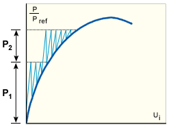
Initial stiffness method

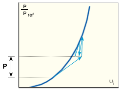
KSTRA=1: Modified Newton-Raphson (MNR)

Here the structure stiffness matrix is updated and factorized at the beginning of each loading increment, that is, at the equilibrium configuration obtained at the end of the previous step (GUID-319C546E-931F-41D8-805E-130A648F79E8.htm#FIG_28C732CA09F04500976FFD3A20E1BCF6 and GUID-319C546E-931F-41D8-805E-130A648F79E8.htm#FIG_1BF645306B304487BB8540E9F54C5736). Iterations are then carried out without reforming the stiffness. This strategy is well suited to those parts of the equilibrium path that are mildly non-linear.

Modified NR method for softening structure

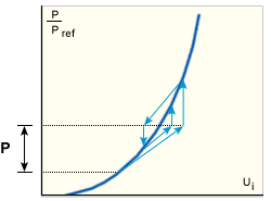
Modified NR method for stiffening structure

KSTRA=2: Combination of NR and MNR

This is a modification of the MNR method in which the stiffness is reformed and factorized at the beginning of the step and again after the first iteration (GUID-319C546E-931F-41D8-805E-130A648F79E8.htm#FIG_BBA0729C970E40F994CC414AB0BCCC08). The algorithm can cope with moderate non-linearities.

Combined method for stiffening structure

KSTRA=3: Newton-Raphson (NR)

In this case, the structure stiffness matrix is updated at the beginning of each iterative cycle (GUID-319C546E-931F-41D8-805E-130A648F79E8.htm#FIG_0A62CC011C5E4F39BDEB04521987A31A). The method exhibits rapid (that is approaching quadratic) convergence and is suitable for dealing with strong non-linearities and bifurcations in the equilibrium path. However, for a given number of iterations, it is clearly the most time-consuming of the alternatives considered so far.

Full NR approach

KSTRA=4: Newton-Raphson (NR) with step reduction

This strategy is identical to KSTRA=3 but is introduced so that when convergence difficulties are encountered using KSTRA 3, the step will be retaken using a quarter of the step size while maintaining pure NR iterations.

KSTRA=5: Load stepping

In this method, equilibrium iterations are temporarily suppressed. Thus, for each load increment, only one reformation and reduction of the structure stiffness is required and no iterations are used (GUID-319C546E-931F-41D8-805E-130A648F79E8.htm#FIG_919CBE47EC1F4BCF85E632871D4044DF). To minimize drift from the true equilibrium path it is essential that the load increments are much smaller those used in MNR or NR and that the unbalanced forces are carried forward (as opposed to being discarded) into the next step. The method is only used as a last resort when all other strategies have failed.

Straight forward load stepping

Equilibrium paths can contain limit points and bifurcations. In the vicinity of such points, the structure stiffness matrix can become ill-conditioned causing even the NR algorithm to fail. However, in such a case it is sometimes possible to successively traverse the difficult section by using load stepping before reverting back to NR. An important feature of the implementation of all the above techniques is that any residual out-of-balance forces remaining at the end of a given step (these will never be identically zero because you must set a target tolerance that is greater than zero) will always be carried forward to the beginning of the next step. In this sense the methods are self-correcting. Compared to methods that discard any residual out-of-balance forces on the basis that they are negligible, the self-correcting scheme leads to higher precision and ensures that there is no accumulative drift away from the true solution path (note that discarding outstanding residuals leads to errors that are tolerance dependent and also accumulate step-by-step). As explained in the section Equilibrium Equations on Page 23, during a successful set of iterative cycles, both the out-of-balance forces and the iterative change in the nodal displacements will tend to zero as the structure settles into its equilibrium configuration. Consequently, the iterative process can be terminated by applying a convergence tolerance to either the residual forces, or to the iterative changes in displacement, or to a combined (energy) measure. The analysis bases its convergence on the following displacement criterion:

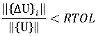
where is the Euclidean norm of the change in nodal displacements between two successive iterations, that is:

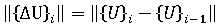
and is the Euclidean norm of the current total nodal displacements. The appropriate value of RTOL to use is somewhat problem-dependent, but values that lie in the range 0.01 to 0.0001 can be expected to provide adequate precision.

Automatic Control Techniques

One of the main difficulties with non-linear finite element analysis is that no single iterative method is best suited to the entire solution path. When the non-linearity of the path becomes more severe, the selected strategy may fail to converge, making further progress impossible. Clearly what is needed is an automatic control system that is capable of retaking a step that has failed using either a different step size and/or a different strategy. Such a scheme is available in the analysis and has been found to be very successful in allowing solution paths to be traced automatically without your intervention. The features of the scheme are as follows:

• You select an initial minimum strategy (normally KSTRA=1 or 2) and an initial step size. This strategy will be maintained until convergence difficulties (if any) are encountered.
• Convergence difficulties are deemed to occur when:
  • convergence has not been achieved in the maximum permitted number of iterations I_max (the default value or specified by you), or
  • the solution is diverging (a divergent solution is assumed if, for iteration 4 or higher, the norm of the current displacement increment, , is greater than the norm of the first displacement increment of the step . Euclidean norm of the out-of-balance forces is greater than the Euclidean norm of the applied loads).
• The solution methods are arranged in order of increasing values of KSTRA. When convergence difficulties are encountered, the program will retake the step using the next higher strategy. Simultaneously the step size is reduced to a quarter of its previous value. The new strategy is now maintained until further convergence difficulties occur in which case the next higher strategy is selected and the step size is again reduced.
• The process will continue until either the maximum number of steps is reached or the load exceeds an allowable level (both these parameters can be adjusted by you).
• Once any strategy that is higher than that originally selected is in use an attempt will be made to return to the next lower strategy provided:
  • four steps of the current strategy (KSTRA = 1, 2, 3 or 4) did not require more than half of the permitted number of iterations, or
  • the current strategy (KSTRA = 5) has been used four times.

If the selected lower strategy fails, then the previous method will be used for a further four increments but without additionally reducing the step size.

Another important feature of the control system is that the step size, , is adjusted dynamically to reflect the degree of difficulty that was experienced in the previous step. The idea is to ensure that the step size decreases in regions of increasing non-linearity and increases in regions of decreasing non-linearity. To achieve this we use the relations:

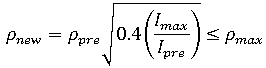
where is the number of iterations used in the previous step, is the maximum number of iterations, and is the step size limit (which can be adjusted by you). As an example, assume that = 1, = 20, = 4, and = 2. Then, from the formula we find that the current step size will be .

This also shows that, following a convergence failure, it will take four steps with an average of 4 iterations in each before the original step size (that is, the step size that was in use in the increment that failed) is recovered. Note that when exceeds 40% of , the step size will contract, albeit relatively slowly.