Membrane elements are three- or four-node elements formulated in three-dimensional space. Membrane elements are used to model fabric-like objects such as tents or cots, or structures such as the roof of a sports stadium. Membrane elements model solids of a specified thickness which exhibit no stress normal to the thickness. The constitutive relations are modified to make the stress normal to the thickness zero.
Determination of Surface Number
Surface-based loads (such as pressure) are applied to the membrane elements by selecting the surface to be loaded. Since each edge of the element could be on a different surface number, the rule for applying surface-based loads to the element is as follows: the load assigned to the highest surface number of all the lines that form the element will be applied to the entire element. If the highest surface number on the element has no applied load, the element will have no applied load. Some care is suggested when determining which surface number to use for the lines between elements with loads and elements without loads.
Degrees of Freedom
Membrane elements, by definition, have only three translational degrees of freedom (DOFs): Dx, Dy, and Dz. They do not have rotational degrees of freedom (DOFs), so they do not transmit moments or give rotation results.
The membrane element allows the definition of pressure loads normal to the surface, for example, to model wind loads on a sail. The convergence of the element for this type of loading is improved if the element is in tension, otherwise the element is free to flap around and convergence difficulties may arise. Temperature-dependent, anisotropic material properties can be defined. Stress output is provided at the nodes.
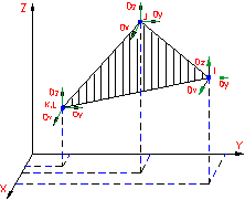
Figure 1: Membrane Element (Triangular)
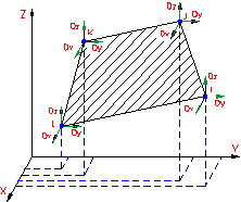
Figure 2: Membrane Element (Quadrilateral)
Membrane Element Parameters
First, you must specify the material model for this part in the Material Model drop-down box. The available membrane material models are:
- Isotropic: This material model option is used for parts that will only experience deflections in the elastic region of the stress-strain curve. To use this material model, the parts must have identical material properties in all directions. A single modulus of elasticity and Poisson's ratio will be the requested material properties.
- Orthotropic: This material model option is used for parts that will only experience deflections in the elastic region of the stress-strain curve. The part may have different material properties in certain directions. Specifically, the material properties may be different in one or more of the three orthogonal directions in a rectangular coordinate system. See the paragraph Controlling the Orientation of Membrane Elements below for details on setting up the material axes.
- Composite: This material model is used to model composite materials in which multiple laminae affect the material properties. The material must remain in the elastic region of the stress-strain curve during the analysis and the material properties must be identical at all temperatures. You will be requested to define the material properties and failure criteria for each layer of the composite in the Composite tab. See the paragraph Controlling the Orientation of Membrane Elements below for details on setting up the material axes.
- Mooney-Rivlin: This material model is used to model hyperelastic materials such as rubber.
- Ogden: This material model is used to model hyperelastic materials such as rubber.
- Viscoelastic Mooney-Rivlin: A viscoelastic variation of the Mooney-Rivlin (hyperelastic) material model.
- Viscoelastic Ogden: A viscoelastic variation of the Ogden (hyperelastic) material model.
Specify the thickness of the membrane elements in the Thickness field. The element is considered to be drawn at the midplane of the membrane element. You must enter a value for the thickness to run the analysis. If the Composite option is selected in the Material Model drop-down box, this field will not be available. In this case, the sum of the thicknesses of the laminae defined in the Composite tab will be displayed in this field.
For the membrane elements in this part to have the midside nodes activated, select the Included option in the Midside Nodes drop-down box. If this option is selected, the membrane elements will have additional nodes defined at the midpoints of each edge. (For meshes of CAD solid models, the midside nodes follow the original curvature of the CAD surface, depending on the option selected before creating the mesh. For hand-built models and CAD model meshes that are altered, the midside node is located at the midpoint between the corner nodes.) This will change a 4-node membrane element into an 8-node membrane element. An element with midside nodes will result in more accurately calculated gradients. Elements with midside nodes increase processing time. If the mesh is sufficiently small, then midside nodes may not provide any significant increase in accuracy.
 Model SetupParametersAdvanced dialog on the Output tab. (See the page Setting Up and Performing the Analysis: Nonlinear: Analysis Parameters: Advanced Settings: Controlling the Output Files for details.)
 Composite Material Model
If the membrane elements are using a composite material model, you can select a failure criteria using the Failure Criterion drop-down box in the Composite tab of the Element Definition dialog. The available options and the corresponding equations used are:
- Tsai-Wu: If this option is selected, the Tsai-Wu (or quadratic tensor polynomial) criteria will be used to determine if the part fails the structural analysis. This criteria, considering the interaction between stresses in two directions, for an orthotropic layer under plane stress condition, is determined by the equation:
|
|
where
![]()
![]()
![]()
![]()
![]()
X t = Axial or longitudinal strength in tension (>0)
X c = Axial or longitudinal strength in compression (>0)
Y t = Transverse strength in tension (>0)
Y c = Transverse strength in compression (>0)
S = Shear strength
F12 = the stress interaction value entered in the material properties. If the value is 0, it will default to![]() .
.
σ 1 = Stress in principal material 1- direction
σ 2 = Stress in principal material 2- direction
τ 12 = Shear stress in principal material 1-2 plane
If equation (1) is not satisfied, the material has failed.
![]() (2)
(2)
where R is the strength/stress ratio.
Since each combination of stress components in (1) reaches its maximum when the left-hand side reaches unity, (2) can be substituted into (1) and yield:
![]()
Solving this equation for R yields:
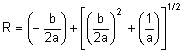
where:
![]()
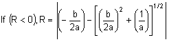
with the signs of the stresses σ ij reversed.
- Maximum Stress: If this option is selected, the maximum stress criteria will be used to determine if the part fails the structural analysis. The criteria is given as:
|
|
 (3)
(3) where
σ 1 = Calculated stress in 1 direction
σ 2 = Calculated stress in 2 direction
τ 12 = Calculated shear stress
X c = Allowable compressive stress in 1 direction (>0)
Yc = Allowable compressive stress in 2 direction (>0)
X t = Allowable tensile stress in 1 direction (>0)
Y t = Allowable tensile stress in 2 direction (>0)
S = Allowable shear stress (>0)
If the conditions of equation (3) are not satisfied, the material has failed.
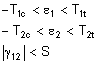
- Maximum Strain: If this option is selected, the maximum strain criteria will be used to determine if the part fails the structural analysis. The criteria is given as:
|
|
 (4)
(4) where
ε 1 = Calculated strain in 1 direction
ε 1 = Calculated strain in 2 direction
γ 12 = Calculated shear strain
T 1c = Allowable compressive strain in 1 direction (>0)
T 2c = Allowable compressive strain in 2 direction (>0)
T 1t = Allowable tensile strain in 1 direction (>0)
T 2t = Allowable tensile strain in 2 direction (>0)
S = Allowable shear strain (>0)
If the conditions of equation (4) are not satisfied, the material has failed.
The Composite Laminate Stacking Sequence table can be used to define the layers of the composite. Layers are oriented and ordered as described below in Controlling the Orientation of Membrane Elements. The Thickness column must be defined for each layer. The Orientation Angle column gives the angle α between the material axes (defined on the General tab) and the fiber or layer axes. The material properties are entered according to the layer axes. To define the material properties for a layer, click in the Material column. A dialog will appear that will allow to select an existing material or Add a new material. (Also see the page Setting Up and Performing the Analysis: Nonlinear: Material Properties: Composite Material Properties for details.)
Control Orientation Membrane Elements
There are two types of axes that the user can control. One type is the axis normal to the membrane elements. The main reason to specify the normal direction is for applying pressure to the element or specifying surface-to-surface contact. For composites, the normal direction controls which side of the element layer 1 is on. The second type of axes is the element's in-plane axes. This is useful when working with an orthotropic material model or you desire to get results in the element coordinate system.
In addition to these two types, there are three axis systems which the user may need to set:
- The element axes.
- The material axes, which is used for orthotropic and composite material models.
- The laminate axes, which is used with composite material models.
Element Axes:
An element normal point is used to control the orientation of the element's normal axis (+3), or which side of the element is the top side (+3 side) and the bottom side (-3 side). The normal direction is determined by specifying a point in space using the X Coordinate, Y Coordinate and Z Coordinate fields in the Element Normal section of the Orientation tab. See Figure 3. A positive normal pressure will be applied normal to the membrane elements the direction of the +3 axis and thus will point away from the element normal point.

|
| Figure 3: Determining the Element Normal The edge-on view of the membrane element is shown. |
For a general FEA analysis, you can ignore the element's in-plane orientation, axes 1 and 2. The ability to orient element's in-plane axes is useful for elements with orthotropic material models and composite elements. The orientation of the 1 and 2 axes is done in the Orientation tab of the Element Definition dialog. The Method drop-down box contains three options that can be used to specify which side of the element will be the ij side. The element axis 1 will be parallel to the ij side of the element. (Element axis 2 forms a right-hand system with axes 1 and 3.)
- If the Default option is selected, the side of an element with the highest surface number will be chosen as the ij side.
- If the Orient I Node option is selected, a coordinate must be defined in the X Coordinate, Y Coordinate, and Z Coordinate fields. The node on an element that is closest to this point will be designated as the i node. The j node will be the next node on the element following the right-hand rule about the element's normal axis (+3 axis).
- If the Orient IJ Side option is selected, a coordinate must be defined in the X Coordinate, Y Coordinate and Z Coordinate fields in the Nodal Order section. The side of an element that is closest to this point will be designated as the ij side. The i and j nodes will be assigned so that the j node can be reached by following the right-hand rule about the element's normal axis (+3 axis) along the element from the i node.
Material Axis:
The material properties are entered in terms of the material axes for orthotropic materials, and the material axes can be defined from the element axes (or from a global reference) using the Material Axis Direction section of the General tab on the Element Definition dialog. (Material properties for composite materials are entered in terms of the layer axes, as described below.)
In all cases, the material axis 3 will be perpendicular to element and in the same direction as the element axis 3.
- If the Element option is selected in the Method drop-down box, the material axes will be based off of the element local axes. Unless modified with the In-plane Rotation Angle, the material 1 and 2 axes will be parallel to the element 1 and 2 axes.
- If the Global X-axis option is selected, the projection of the global X axis onto the element creates the material axis 1.
- If the Global Y-axis option is selected, the projection of the global Y axis onto the element creates the material axis 1.
- If the Global Z-axis option is selected, the projection of the global Z axis onto the element creates the material axis 1.
- If the Point option is selected, a point will be defined in the X Coordinate, Y Coordinate and Z Coordinate fields. The material axis 1 will be in the direction from the user-defined point to each integration or gauss point (and projected into the plane of the element). Essentially, this places axis 1 in a radial direction. Material axis 2 is in the plane of the element and forms a right-hand system with axes 1 and 3.
- If the Vector option is selected, a vector will be defined using the X Coordinate, Y Coordinate, and Z Coordinate fields. The material axis 1 is then parallel to the defined vector. Material axis 2 is in the plane of the element and forms a right-hand system with axes 1 and 3.
Regardless of the method used to orient the membrane element material axes, you can use the In-Plane Rotation Angle field to rotate the material axes by a specified angle about axis 3. The rotations follow the right-hand rule about axis 3. See Figure 4.
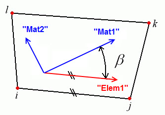
Figure 4: Rotation Angle Definition of Material Axis Direction
The Element method of setting the material axis is shown in which the angle β is measured from the element 1 axis.
Layer Axes:
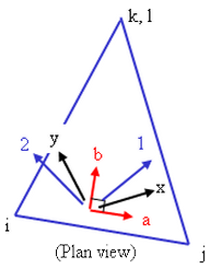
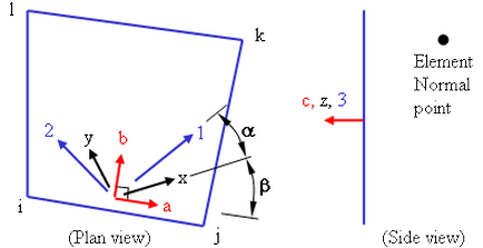
For composites, each layer of the laminate has a set of local axes. The layer 1-axis is the axis along the fiber of each individual layer. The layer 2-axis is the axis perpendicular to the fiber of each individual layer and in the plane of the element. The layer 3-axis is perpendicular to the element and therefore parallel to the local element axis c. (To avoid confusion between the layer axes and the element axes, the element axes are often referred to as a-b-c when working with composites, and axes 1-2-3 define the orientation of the fibers.) See Figures 5 and 6.
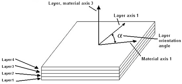
Figure 5: Laminae Stacking Order
The user enters the angle a for each layer using the Orientation Angle of the Composite Laminate Stacking Sequence table. Axis 3 is controlled by the element normal coordinate.
|
|
Figure 6: Alternate Depiction of Element, Material, and Layer Axes
The element axes a-b-c are based off of the element normal coordinate and the ij side of the element. The material axes x-y-z are rotated an angle β from the element axes. The element and material axes are the same for all layers in the stack. The layer or fiber axes 1-2-3 are rotated an angle from the material axes and can be different angles for each lamina in the stack. |
Advanced Membrane Element Parameters
Select the formulation method that you want to use for the membrane elements in the Analysis Formulation drop-down box in the Advanced tab. The Linear option will ignore nonlinear geometric effects that result from large deformation. The Geometrically nonlinear option will include nonlinear geometric effects that result from large deformation.
If the Allow for overlapping elements check box is activated, overlapping elements will be allowed to be created when the lines are decoded into elements. Overlapping may be necessary when modeling elements. This is especially true for problems confined to planar motion.
For the stress results for each element to be written to the text log file at each time step during the analysis,. activate the Detailed stress output check box. This may result in large amounts of output.
Membrane elements use selective reduced integration to alleviate locking problems. If the Reduced integration for membrane shear terms check box is activated, membrane locking behavior for curved element configurations will be improved.
If the No compression check box is activated, and element that is under compression will have no stiffness applied to it. This will enable the modeling of sails and similar parts.
Basic Steps for Use of Membrane Elements
- Be sure that a unit system is defined.
- Be sure that the model is using a nonlinear analysis type.
- Right-click the Element Type heading for the part that you want to be membrane elements.
- Select the Membrane command.
- Right-click the Element Definition heading.
- Select the Edit Element Definition command.
- In the General tab, select the appropriate material model in the Material Model drop-down box.
- Enter the Thickness of the shell elements. This is required information and the model will not run without it being entered.
- If the Composite option is selected in the Material Model drop-down box, specify the appropriate data in the Composite tab.
- Click the Orientation tab.
- Specify an element normal point. The top of the membrane element will always point away from this point.
- Press the OK button.