Current Results
When you select Results Inquire  Inquire Current Results, the Inquire : Results dialog will appear. Depending on the type of result being displayed, select a node, element, or face to display the current result. Nodal results (displacements, stresses, temperatures, and so on) will show the coordinates of the node (undisplaced and displaced coordinates if appropriate), the elements in which that node is used (when displaying an element-based result, such as stress), and the current result contour value. Element results (heat fluxes, and so on) will give the element number and current result contour value. Face results (heat flow rate, and so on) will give element and face number and the current result contour value. The results include all smoothing settings.
As you click a different object (nodes or elements or faces), the information in this screen will update to reflect the currently selected object. If you hold down the Ctrl key, the information for the next item will be added (in ascending order) to the current display.
- For some results, if you select an element then all the nodes on the selected element will be displayed in the Inquire: Results dialog. In all cases, you can select an item, right-click, and choose Select Subentities and choose a subset to be selected.
- Also see the page Results Environment for a discussion of how the results are displayed based on various settings, such as nodal-based versus element-based result, hidden versus not hidden elements, smoothing on versus smoothing off, and so on. In all cases, you can select an item, right-click, and choose Select Subentities and choose a subset to be selected.
- Show or Hide Element Results on Hidden Elements: When displaying an element-based result, such as stress, the Inquire: Results window will list the elements used by the selected node. When the Include results from hidden elements check box is activated, the list of elements include both visible and hidden elements, and therefore the Current Result Value shown also includes the contribution from these hidden elements. When the Include results from hidden elements option is deactivated (unchecked), the list of elements and the current result value are only from the visible elements.
- Summary: By changing the option in the Summary drop-down box, you can have the results for the currently selected nodes manipulated by several methods. The available options are the following:
- None: Displays no summary result.
- Maximum: Displays the maximum result. By definition, a positive value is larger than a negative value, so the positive value would be displayed regardless of the magnitudes.
- Maximum Magnitude: Displays the value for the result with the maximum magnitude. For example, if the results of two selected nodes are 0 and -5, -5 would be displayed in the summary.
- Mean: Displays the arithmetic average of the results, the sum of Ri divided by number of nodes. (see Definitions below.)
- Minimum: Displays the minimum result. By definition, a negative value is smaller than a positive value, so the negative value would be displayed.
- Range: Displays the result of the maximum value minus the minimum value.
- Sum. Adds the selected results. This is especially useful when you want to sum the reaction forces over several nodes or when you want to sum the total heat flow through a certain area of a heat transfer model.
- Mean Weighted By Volume: Displays the average of the results for the selected elements, weighted by the volume of the elements, the sum of (Ri x Vi) divided by sum of Vi. (see Definitions below.)
- Mean Weighted By Mass: Displays the average of the results for the selected elements, weighted by the mass of the elements, the sum of (Ri x mi) divided by sum of mi. (see Definitions below.)
- Equilibrium Temperature: Displays the average temperature of the selected elements, weighted by mass and specific heat. To compute this summary result, the analysis type must be a heat transfer analysis, the results display must be set to temperature, and the material properties need to include the mass density and specific heat. In most situations, the equilibrium temperature can relate to the enthalpy of the part or system; thus, calculating the equilibrium temperature at two states is equivalent to calculating the change in enthalpy.
The equilibrium temperature can be thought of as the temperature at which the selected elements would obtain if they were allowed to come to equilibrium, without losing any heat to the environment. It is based on the following methodology:
integral of (mi x Cpi x dT) divided by integral of (mi x Cpi), both integrated over the range of Ti to Tequil.
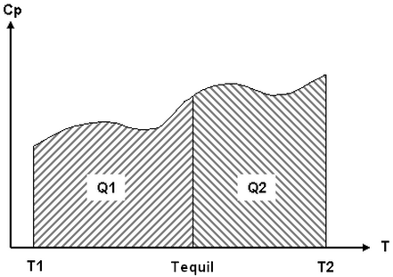
This is easy to visualize for a two mass system. The heat lost by one mass (integral of m2 x Cp2 x dT over the range T2 to Tequil) is equal to the heat gained by the other mass (integral of m1 x Cp1 x dT over the range of T1 to Tequil), so the areas under the graph of specific heat versus temperature are equal. See Figure 1.
|
|
|
The equilibrium temperature Tequil is the temperature at which the amount of heat lost by one mass, Q2, equals the heat gained by another mass, Q1. The area under the curve of the specific heat Cp versus the temperature T is equal for Q1 and Q2. |
|
Figure 1: Equilibrium Temperature Calculation for Two Masses |
Definitions used in the summary calculations
- Cpi is the specific heat of the element at node i. Naturally, the specific heat must have been entered in the material properties in order for this calculation to give a meaningful result.
- mi is the mass of the element at node i. The mass of the element is assumed to be equally distributed to all the nodes. Naturally, the mass density must have been entered in the material properties in order for this calculation to give a meaningful result.
- Ri is the result at node i.
- Tequil is the equilibrium temperature.
- Ti is the temperature at node i.
- Vi is the volume of the element at node i. The volume of the element is assumed to be equally distributed to all the nodes on the element.
-
- For the options that require elements to be selected, keep in mind that all the nodes on the selected elements will be selected, displayed in the Inquire: Results dialog, and therefore considered in the summary calculation.
- Shape functions are not used in computing the weighted results or the equilibrium temperature. The mass, volume, specific heat, and result are simply divided equally among the nodes of the element. For elements without midside nodes, this method will produce accurate results. For elements with midside nodes, the results are reasonable.
- The weighted results for composite elements are based on the mass and volume of the entire element, not on each layer individually. When viewing the results of a single layer, the weighted result may not be meaningful.
- Clear Contents: Pressing this button will clear the current information from the Inquire: Results screen.
- Save Values: This option will allow you to save the current data to a text file. The .out format will create a text file similar in format to the Inquire: Results dialog. The .csv format will create a comma-separated value file where each item on the row is separated by a comma; this format is convenient for importing into a spreadsheet and using the data for other purposes.
The Export Results dialog will appear when the Save Values button is clicked. Choose the file name and location of the exported results. Activate the Append check box on the Export Results dialog before clicking the Save button to append the current results to an existing file. Otherwise, the existing file will be overwritten with the current results.
- Save To Report: This option is similar to the Save Values command in that the results shown in the Inquire: Results windows are saved to a text file. The differences are as follows:
- You can only specify the name of the file.
- The extension is .out.
- The location is set to the ds_inquired_results folder located under the design scenario.
- The text file will be appended to the Report.
- Specify: Pressing the Specify button will present these ways to input specific items to select and display the results for:
- Part Number and Element Number: When viewing element and face-based results, the Specify dialog prompts you for a part number and element number. The element number can include multiple elements by separating them with a comma (,). For example, entering the text 1, 14, 21 (without the quotation marks) in the Element Number field will give the results for element numbers 1, 14, and 21.
- Node Number(s): When viewing nodal-based results, this option on the Specify dialog will allow you to enter a node number for which to view the results. Multiple nodes can be entered by separating them with a comma (,). For example, entering the text 1, 14, 21 (without the quotation marks) in the Node Number(s) field will give the results for node numbers 1, 14, and 21.
- Location: When viewing nodal-based results, this option on the Specify dialog will allow you to enter a coordinate (X,Y, and Z) and Radius. All nodes within the radius of the specified coordinate will be selected. A Radius of zero (0) will select the closest node to the specified coordinate.
Note:- For stress models, displaying the displaced model and exaggerating the displacement scale factor will affect whether a node is within the radius of the specified location. Displaying the displaced shape and exaggerating the displacement scale will change the position of the nodes relative to the specified location. (The displacement scale is controlled by Results Contours Displacement Show Displaced Displaced Options Scale Factor.) In this regards, the Location option is no different than drawing a 3D selection sphere in the display area (if such a thing existed); nodes that appear inside the sphere are selected.
- Naturally, set the displacement scale factor to As an Absolute Value and enter a Scale Factor of 1 to select nodes whose displaced positions are actually within the radius of the specified location.
The nodes or elements will be highlighted in the model, just as if you selected the objects with the mouse. Displaying an unshaded view of the feature lines (View
Appearance Visual Style Features) can help show where the highlighted objects are in the model. - Inquiring on Boundary Element Results: If either the Results Contours Other Results Element Forces Axial Force, Results Contours Other Results Element Forces Axial Moment, Results Contours Other Results Element Displacements Stretch or Results Contours Other Results Element Displacements Twist is selected, you will be able to inquire on the results value for a boundary element by inquiring on the node on the model to which the boundary element is attached. The Inquire: Results dialog list the results for each element in each part of the model that is connected at that node. To determine which part contains the boundary elements, use Results Inquire Inquire Model Statistics . The element type for each part and the amount of elements in each part will be listed. To determine which element number corresponds to which boundary element, use Results Inquire Inquire … Element Information. Press the Specify button, type the part number of the boundary elements in the Part Number field and type a valid element number in the Element Number field. The specified boundary element will become highlighted in the display area. This is useful when more than one boundary element is located at a single node.
Loads and Constraints
When you select this command, the Inquire: Loads and Constraints dialog will appear. Use Selection Select Loads Constraints to limit your selection to the load and constraint objects. To further limit the selection, use the Selection Filter to select which loads and constraints will be available for selection. You can select on any load or constraint and the type of load or constraint, the node or element to which it is applied, the coordinates, and the relevant information will be displayed in the Inquire: Loads and Constraints dialog. As you click more loads or constraints the information in this screen will update to reflect the current selected object. If you hold down the Ctrl key, the information for the next object will be appended to the current display.
Distance and Angle
When you select this command, the Inquire: Distance and Angle screen will appear. This screen gives the following information by clicking on successive points:
- Clicking on two points will give the total distance between the points.
- Clicking on three points (which forms two vectors) will give the angle between the two vectors.
- Clicking on four points (which forms a quad region) will give the fold angle of the quad. Be sure to click in a consistent direction to measure the warp angle: click either clockwise or counter-clockwise. The Fold Angle 1 is calculated by the angle between the vectors normal to the two triangles created by dividing the quadrilateral with a line from the second node selected to the fourth node selected. The Fold Angle 2 is calculated in the same manner but divides the quadrilateral from the first node selected to the third node selected.
Maximum Results Summary
When you select this command, the Inquire: Maximum Results Summary dialog will appear. The dialog window will contain the maximum result, based on the current result contour being displayed, for all nodes in the model, for all load cases or time steps. All nodes includes nodes on hidden parts, on hidden elements, and in the interior of solid or brick element parts. The results are sorted in descending order based on the value of the result.
- Clear Contents: Pressing this button will clear the current information from the Inquire: Maximum Results Summary dialog.
- Save Values: This option will allow you to save the current data to a text file. The .out format will create a text file similar in format to the Inquire: Maximum Results Summary dialog. The .csv format will create a comma separated value file where each item on the row is separated by a comma; this format is convenient for importing into a spreadsheet and using the data for other purposes.
The Export Results dialog will appear when the Save Values button is clicked. Choose the file name and location of the exported results. Activate the Append check box on the Export Results dialog before clicking the Save button to append the current results to an existing file. Otherwise, the existing file will be overwritten with the current results.
Detailed Beam Stress and Strain
When an MES or nonlinear beam element is selected, the Inquire panel includes the options Detailed Beam Stress and Detailed Beam Strain. These commands give the stresses and strains calculated by the processor.
Stress Beam and Truss commands are only partially corrected by the yield strength. Each of the stresses (axial stress, bending stress in local 2, and bending stress in local 3) are capped or limited to the yield stress if necessary. The worst stress then adds the three results together. The format of the information in the Inquire Detailed Beam Stress dialog is as follows:
Part Element Section Intx Inty Intz State S1-1 S1-2 S1-3
where
- Part is the part number
- Element is the element number
- Section is the section number (when cross section is treated as a series of rectangles)
- Intx is the integration point in axial direction (local x-dir or 1 axis) and increments from 1 through the integration order set by the user (7 maximum)
- Inty is the integration point in local y-dir (2 axis) and increments from 1 through the integration order set by the user (7 maximum)
- Intz is the integration point in local z-dir (3 axis) and increments from 1 through the integration order set by the user (7 maximum)
- State indicates whether the point is elastic or plastic
- S1-1 is the normal stress or strain in the 11 direction
- S1-2 is the shear stress or strain in the 12 direction
- S1-3 is the shear stress or strain in the 13 direction
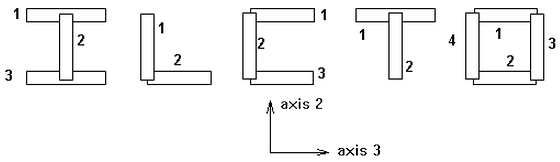
Imagine the beam element composed of numerous integration points in all three directions (axis 1 along the length, axes 2 and 3 in the plane of the cross section). The stress and strain output is given at all the integration points, so with the integration order set to 2x2x2, each element would output 8 lines of results for each element.
Find the 3D position (X, Y, Z) of the integration point (Intx, Inty, Intz) within the element. This is done with the following calculations depending on the shape.
Rectangle
Y = C(Inty,TINTy)*height*0.5, measured from the neutral axis in the direction of axis 2
Z = C(Intz,TINTz)*width*0.5, measured from the neutral axis in the direction of axis 3
Circle
R = radius/2
R = R + C(Inty,TINTy)*R and Shear and Moment Diagrams
α = (2π/TINTz)*(Intz-1)
Y = R*cos(α), measured from the neutral axis in the direction of axis 2
Z = R*sin(α), measured from the neutral axis in the direction of axis 3
Hollow circle
R = (Ro+Ri)/2
R = R + C(Inty,TINTy)*(Ro-Ri)/2
α = (2π/TINTz)*(Intz-1)
Y = R*cos(α), measured from the neutral axis in the direction of axis 2
Z = R*sin(α), measured from the neutral axis in the direction of axis 3
where
- X = C(Intx,TINTx)*0.5*Length+0.5*Length, measured from node i (= node 1)
- TINTx is the total number of integration points in x-dir (Integration Order in local 1 axis)
- TINTy is the total number of integration points in y-dir (Integration Order in local 2 axis)
- TINTz is the total number of integration points in z-dir (Integration Order in local 3 axis)
and the quantity C(i, Integration Order) is from the following table:
| Integration Order | C(i, Integration Order) | ||||||
| i = 1 | i = 2 | i = 3 | i = 4 | i = 5 | i = 6 | i = 7 | |
| 1 | 0 | - | - | - | - | - | - |
| 2 | -1 | 1 | - | - | - | - | - |
| 3 | -1 | 0 | 1 | - | - | - | - |
| 4 | -1 | -0.333 | 0.333 | 1 | - | - | - |
| 5 | -1 | -0.5 | 0 | 0.5 | 1 | - | - |
| 6 | -1 | -0.6 | -0.2 | 0.2 | 0.6 | 1 | - |
| 7 | -1 | -0.666 | -0.333 | 0 | 0.333 | 0.666 | 1 |
General cross section
Each section is treated as an independent quadrangle separately. C(i,j) can be directly applied to find the position.
Predefined cross section
Each section is treated like an independent quadrangle separately as below, with the section number indicated.
Model Statistics
When you select this command, the Inquire: Model Statistics dialog will appear. The number of nodes, elements, load cases and parts will be displayed in the dialog. In addition the details for each part will be shown.
Element Information
When you select this command, the Inquire: Element Information dialog will appear. You can select any element and the element number, element, type, and the nodes that create this element will be displayed in the screen. As you click more elements, the information in this screen will update to reflect the currently selected element. If you hold down the Ctrl key, the information for the next element will be appended to the current display.
Pressing the Specify button will allow you to enter a part number and element number for which to view the element information. Multiple elements can be entered by separating them with a comma (,). For example, entering the text 1, 14, 21 (without the quotation marks) for the Element Number field will select the element numbers 1, 14, and 21 in the designated part.
The element or elements will be highlighted in the model just as if you selected the elements with the mouse. Displaying an unshaded view of the feature lines (View: Display: Features) can help show where the highlighted elements are in the model.
Adding Shear and Moment Diagrams
When beam elements are selected in a stress analysis, the following commands are available in the Results Inquire tab, Graphs panel to draw shear and moment diagrams:
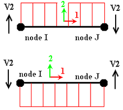
- Add Shear Diagrams (Axis 2): This command will display the diagram of the shear forces along the local axis 2 direction. The diagram is plotted in the plane formed by element axes 1 and 2.
- Add Shear Diagrams (Axis 3): This command will display the diagram of the shear forces along the local axis 3 direction. The diagram is plotted in the plane formed by element axes 1 and 3.
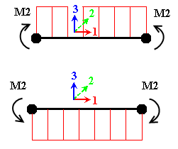
- Add Moment Diagrams (Axis 2): This command will display the diagram of the bending moment about the local axis 2 direction. The diagram is plotted in the plane formed by element axes 1 and 3.
- Add Moment Diagrams (Axis 3): This command will display the diagram of the bending moment about the local axis 3 direction. The diagram is plotted in the plane formed by element axes 1 and 2.
- Clear Beam Diagrams: This command will clear the shear and/or moment diagrams from the selected beam elements.
The diagrams are drawn or removed from the selected beam elements only; other diagrams in the model are not affected. The two shear diagrams cannot be shown simultaneously on the same element, nor can the two moment diagrams be displayed on the same element. One shear and one moment diagram can be shown on the same element.
The direction of the shear and moment diagrams follow the convention shown in the following figures. In the figures, keep in mind that the sign of the values (V2 for shear or M2 for moment) follow the conventions described in the paragraph Element Forces and Moments on the page: Linear Results.
|
|
|
Direction of the Shear Diagram. The arrow at node I controls on which side of the element the diagram is drawn. The shear in the direction of axis 2 is drawn in the plane of axes 1 and 2 (shown above); the shear for axis 3 is drawn in the plane of axes 1 and 3. |
Direction of the Moment Diagram. The arrows control on which side of the element the diagram is drawn. The moment about axis 2 is drawn in the plane of axes 1 and 3 (shown above); the moment about axis 3 is drawn in the plane of axes 1 and 2. |
 Options Results Individual FEA Object Settings to set the color of the Moment Diagram or Shear Diagram.
 Average Film Coefficient
This command is only available for thermal analyses. When this command is selected, the Inquire: Average Film Coefficient dialog will appear.
You can select one or multiple faces of the model. The screen will report the faces that are selected and the average film coefficient, h, over those faces. The equation used to calculate h is:
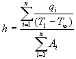
Where: h = Average film coefficient
q = Heat rate of face through face i
T i = Average temperature of the nodes that define face i
![]() = Ambient temperature which must be defined by pressing the Ambient Temperature button
= Ambient temperature which must be defined by pressing the Ambient Temperature button
A i = Area of face i
Probes Panel
Th Probe command will activate probe mode. As you move the mouse over the model, a probe will appear displaying the current result value for that node, element or face (depending on the selection method). If you want the probe to remain on a node, right-click in the display area and select the Add Probe command.
- Also see the page Results Environment for a discussion of how the results are displayed based on various settings.
- The number of decimal points displayed by the probe can be controlled from the Result Contours Settings Legend Properties Probe Settings command. See the page: Probe Settings Tab for details.
The Maximum and Minimum commands display a pointer at the nodes with the maximum and minimum current result value, respectively. Optionally, activate the Minimum Maximum Nodes option to append the node number to each probe. This option is in the pull-out section of the Probes panel.
Lastly, in the pull-out section of the Probes panel, there is a Contact Diagnostic Probes option, which is enabled by default. These diagnostic probes indicate where penetration or chatter are occurring during a surface contact analysis. Click this option to toggle the visibility of the contact diagnostic probes.