Linear Results

None

Selecting this option will remove any results contour from the model and will use the default colors for the shading and the mesh lines.

Displacement

This option will color the model to display the displacement. The commands available are as follows:

Magnitude Sets the display to be based on the magnitude of the displacement. This will always be a positive value. The magnitude is the total distance the node has move. mag = sqrt[(dX)^2 + (dY)^2 + (dZ)^2]
X Sets the display to be based on the dot product of the displacement vector with a unit vector in the X direction. It shows the component of the total displacement in the X direction.
Y Sets the display to be based on the dot product of the displacement vector with a unit vector in the Y direction. It shows the component of the total displacement in the Y direction.
Z Sets the display to be based on the dot product of the displacement vector with a unit vector in the Z direction. It shows the component of the total displacement in the Z direction.
Vector Plot Sets the display to be based on the magnitude of the displacement, showing the result as a vector (arrow) drawn at each node. The length and color of the arrow represent the magnitude of the displacement, and the direction of the arrow represents the vector direction of the displacement. Use the Display Options: Plot Settings: Vector Plots tab to adjust the arrow sizes.

Rotation

This option will color the model to display the rotation at each node. This result will only be valid for nodes on elements that can resist rotation. For example, the nodes on brick elements only have the three translational degrees of freedom available. Therefore the rotational displacement will not be calculated. Nodes on beam elements can resist all three rotations. Nodes on plate elements can resist the two in-plane rotations. The commands available are as follows:

Magnitude Sets the display to be based on the magnitude of the rotational displacement. This will always be a positive value. The magnitude is the total rotation the node has moved. mag = sqrt[(rX)^2 + (rY)^2 + (rZ)^2]
X Sets the display to be based on the dot product of the rotation vector with a unit vector in the X direction. It shows the component of the total rotation about the X axis.
Y Sets the display to be based on the dot product of the rotation vector with a unit vector in the Y direction. It shows the component of the total rotation about the Y axis.
Z Sets the display to be based on the dot product of the rotation vector with a unit vector in the Z direction. It shows the component of the total rotation about the Z axis.

The rotation results need to be interpreted with care in a large deflection analysis (MES or nonlinear analysis) when multiple rotations are involved. The rotation results include the complete history of the motion and therefore are path dependent. See the following figure for an example. (The displacement results are not path dependent.)

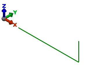An L shaped beam starts in the XZ plane.

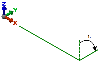First, the beam is rotated -90 degrees about the X axis.

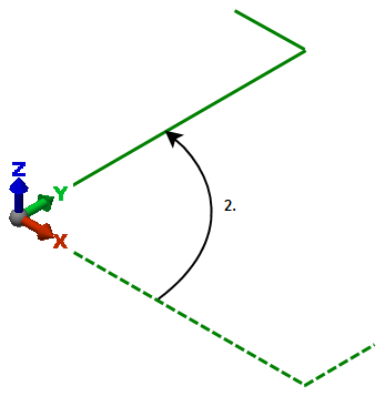Second, the beam is rotated 90 degrees about the Z axis.

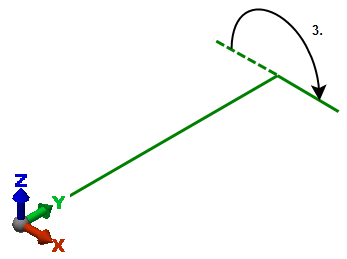Third, the beam is rotated 180 degrees about the Y axis.

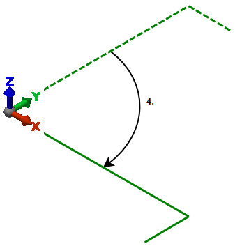Fourth, the beam is rotated -90 degrees about the Z axis.

Comparing the final position with the initial position, it seems that the final rotation results would be a net of +90 degrees about the X axis and 0 degrees about the Y and Z. In large deflection analyses, the results are -90 degrees about X, 180 degrees about Y, and 0 degrees about Z.

Since the displacement results are path independent, the final displacement results are 0 in X, -L in Y and Z, where L is the length of the short leg.

In the above example, the difference between using the Large rigid body rotation option (set on the beam element's Element Definition dialog) is the visualization of the beam's orientation. The orientation of axes 2 and 3 are accurate only when using the large rigid body rotation.

Normalized Displacement and Rotation

For the following two linear analysis types:

Natural Frequency (Modal)

Displacement results – both translational and rotational – are normalized. The sole purpose of these results is to show the deformed shape of the model for each vibration mode. Since the displacements are not scaled to any specific excitation, the absolute displacement and rotation values have no meaning.

Stress

Various analytical techniques are available to assist you in determining the suitability of your model. The Results environment provides access to many of these techniques by providing both the raw stresses in local coordinates and many quantities derived from these raw stresses. Derived quantities include von Mises and Tresca criteria, maximum and minimum principal stresses, and element-specific output. Since the accuracy of the analytical results depends on the construction of the mesh and the application of FEA parameters, the Results environment provides a precision estimate at shared nodes. This precision value can assist you in determining the suitability of your model.

Calculations

The software uses the stress-to-nodes method for calculating stress estimations. Using an extrapolation scheme, calculations using nodal stresses usually provide greater accuracy than calculations derived from the stresses inside the elements. Displaying stresses at nodes produces a more realistic and convenient representation of a model under load, because stress values at nodes are more useful than stress values calculated for whole elements.

Stresses calculated for elements produce stress information at Gaussian points. Gaussian points are the numerical integration points at which the finite element solution and the theoretical solution are most similar. The older technique averaged these stresses to center or faces of 2D elements and the centroid of 3D elements, and can show relatively large differences between adjoining elements. Because finite element solutions are approximations of a continuous function, the results from these locations may be too coarse to provide accurate pictures of how a model behaves under stress.

Calculating stresses at individual nodes corrects this problem. Using the 'local-least-squares' method, stresses are extrapolated from Gaussian points to associated nodes. Accurate assessments of stresses at nodes are especially important when nodes are on the surface or edges of the part being analyzed, since these nodes generally coincide with critical areas of the model. Accuracy information is also available where nodes are shared between different elements.

When displaying the surface of a model, the intensity or stress at each point in each element of the mesh that defines the surface, is calculated, and an appropriate displaying value is assigned to that point. Next, the scale used to display the surface is examined, and the appropriate colors and shades for each point are selected, based on the value calculated at that point. The model is then redrawn with its surface shaded according to the displaying technique used. The Results environment provides visualization options, such as smoothing, to let you control the way your model is displayed. This lets you visualize your model in the way that is most significant to you.

von Mises

This command sets the results display to be the equivalent von Mises stress for a display or data output. The von Mises stress can be displayed for element types with area (2D, plates, and so on) and volume (bricks).

The equation used is:

where S_x, S_y, and S_z are the axial stresses in the global directions, and S_xy, S_yz, and S_xz are the shear stresses. In terms of the principal stresses S₁, S₂ and S₃:

Note by the equations that the von Mises value is always positive.

Tresca*2

The Tresca*2 stress can be displayed for element types with area (2D, plates, and so on) and volume (bricks). This method extracts the maximum shear stress from the following stress tensor. The Tresca equation is:

where S1, S2, and S3 are the principal stresses. The value reported is twice the maximum shear stress. Thus yielding would occur when the reported Tresca*2 value reaches the yield stress. By definition, the Tresca stress is always positive. See Mohr's Circle for an illustration of this. Tresca*2 is also known as the stress intensity.

Minimum Principal

This command sets the results display to calculate the minimum principal stress (S3) for displaying or data output. The principal stress can be displayed for element types with area (2D, plates, and so on) and volume (bricks). Positive (+) indicates tension, and negative (-) indicates compression. See Mohr's Circle for an illustration of this.

Minimum Principal Direction

This command will display a vector plot of the direction of the minimum principal stress in each element. The tensors at each node of the element are averaged and the minimum principal direction of this average tensor is plotted at the element centroid. If you select an element and select Results Inquire Inquire Current Results, the components of this vector will be displayed.

Intermediate Principal

This command sets the results display to calculate the intermediate principal stress (S2) for displaying or data output. This is the stress in the direction normal to the minimum and maximum principal stresses. The principal stress can be displayed for element types with area (2D, plates, and so on) and volume (bricks). Positive (+) indicates tension, and negative (-) indicates compression.

Intermediate Principal Direction

This command will display a vector plot of the direction of the intermediate principal stress in each element. The tensors at each node of the element are averaged and the intermediate principal direction of this average tensor is plotted at the element centroid. If you select an element and select Results Inquire Inquire Current Results, the components of this vector will be displayed.

Maximum Principal

This command sets the results display to calculate the maximum principal stress (S1) for displaying or data output. The principal stress can be displayed for element types with area (2D, plates, and so on) and volume (bricks). Positive (+) indicates tension, and negative (-) indicates compression. See Mohr's Circle for an illustration of this.

Maximum Principal Direction

This command will display a vector plot of the direction of the maximum principal stress in each element. The tensors at each node of the element are averaged and the maximum principal direction of this average tensor is plotted at the element centroid. If you select an element and select Results Inquire Inquire Current Results, the components of this vector will be displayed.

Tensor

This command displays the component of the stress in the chosen direction. Technically, it uses the double dot product with the stress tensor or local stress components. The stress tensor can be displayed for element types with area (2D, plates, and so on) and volume (bricks).

If Results Contours Settings Use Element-Local Results is not active, you will be able to select between the following global stresses. If this option is active, the following choices will display the local stress tensors mentioned in the individual descriptions.

For elements with local axes, smoothing (averaging) the stresses may not be meaningful, especially if the orientation of the local axes varies between adjacent elements. The smoothed stress tensor values are meaningful only if the local axes are in a consistent direction from one element to the next element.

1) XX Stress tensor component showing the normal stress in the global X direction. Positive (+) indicates tension; negative (-) indicates compression. If Results Contours Settings Use Element-Local Results is active, the local 1-1 stress tensor will be displayed.
2) YY Stress tensor component showing the normal stress in the global Y direction. Positive (+) indicates tension; negative (-) indicates compression. If Results Contours Settings Use Element-Local Results is active, the local 2-2 stress tensor will be displayed.
3) ZZ Stress tensor component showing the normal stress in the global Z direction. Positive (+) indicates tension; negative (-) indicates compression. If Results Contours Settings Use Element-Local Results is active, the local 3-3 stress tensor will be displayed.
4) XY Stress tensor component showing the shear stress in the global XY direction. (X indicates the direction normal to the face, and Y indicates the direction of the shear stress.) If Results Contours Settings Use Element-Local Results is active, the local 1-2 stress tensor will be displayed.
5) YZ Stress tensor component showing the shear stress in the global YZ direction. (Y indicates the direction normal to the face, and Z indicates the direction of the shear stress.) If Results Contours Settings Use Element-Local Results is active, the local 2-3 stress tensor will be displayed.
6) ZX Stress tensor component showing the shear stress in the global ZX direction. (Z indicates the direction normal to the face, and X indicates the direction of the shear stress.) If Results Contours Settings Use Element-Local Results is active, the local 3-1 stress tensor will be displayed.

Beam and Truss

This command will show the stresses for linear and nonlinear truss elements, linear and nonlinear beam elements, and nonlinear pipe elements. The results available are the following:

Attention:

For nonlinear analyses with beam elements that experience plasticity, the results shown by these commands are only partially corrected by the yield strength. Each of the stresses (axial stress, bending stress in local 2, and bending stress in local 3) are capped or limited to the yield stress if necessary. The worst stress then adds the three results together.
For a more accurate stress result, activate the Binary stress and strain output option on the beam's Element Definition before running the analysis. Then use Results Inquire Inquire Detailed Beam Stress and Results Inquire Inquire Detailed Beam Strain in the Results environment to review the results.

Axial Stress (Local 1 Direction): Displays the axial stress. This is calculated by dividing the axial force by the cross sectional area. A positive value indicates tensile stress, and a negative value indicates compressive stress.
Bending Stress in Local 2 Direction: Displays the bending stress in beam elements due to bending moment about the local 2 axis. This is calculated by dividing the bending moment about axis 2 by the section modulus about local axis 2. The local 2 axis passes through the k-node and is perpendicular to the beam. (Since truss elements have no bending capability, this menu item does not apply to truss elements.)
Bending Stress in Local 3 Direction: Displays the bending stress in beam elements due to bending moment about the local 3 axis. This is calculated by dividing the bending moment about axis 3 by the section modulus about local axis 3. The local 3 axis is the cross product of the local 1 and local 2 axes. (Since truss elements have no bending capability, this menu item does not apply to truss elements.)
Worst: At one corner, the combination of axial stress, bending stress about axis 2, and bending stress about axis 3 produces the largest absolute value. This is the worst stress in the beam. For Linear Stress, positive (+) indicates the beam is in axial tension, and negative (-) indicates the beam is in axial compression. Mathematically,

Worst = (sign of P/A)(ABS(P/A)+ABS(M2/S2)+ABS(M3/S3))

A stress analysis (both linear and nonlinear) assumes the cross section is symmetric (due to only one input or calculated value for S2 and S3). Therefore, the worst stress could mathematically occur at a nonexistent location in a nonsymmetrical beam, such as in the lower-left or upper-left corner of Figure 1.

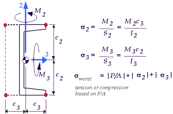
Figure 1: Stress Results in a Nonsymmetrical Beam

Because C2 and C3 are assumed to be equal (based on only one input for S3 and S2), the worst stress can be reported at a nonexistent location.

Use Results Options View Element Orientation to display the local 1, 2, or 3 axes for the beam elements.

Composite

Failure Index

This command will display the results corresponding to the in-plane composite failure criteria set in the Element Definition dialog (Tsai-Wu, Maximum Stress or Maximum Strain).

It is recommended that smoothing (Results Contours Settings Smooth Results) be turned off to see the actual failure criteria value in each element (instead of the smoothed or averaged value between adjacent elements).

You can control the lamina for which you are viewing the results using Results Contours Stress Composites Options. You can also choose to view the Worst results using this command.

For the maximum stress and maximum strain criteria, first consider the following factors of safety, based on the top and bottom surface of the laminae:

Maximum Stress - Factors of Safety:

,,,,and

where σ is the calculated normal stress in direction 1 or 2, X and Y are the allowable stresses in direction 1 and 2 (compression or tension matched to the calculated stress), τ₁₂ is the calculated shear stress, and S is the allowable shear stress.

Maximum Strain - Factors of Safety:

,,,, and

where ε is the calculated normal strain in direction 1 or 2, T is the appropriate allowable strain in direction 1 and 2 (compression or tension matched to the calculated strain), γ₁₂ is the calculated shear strain, and S is the allowable shear strain.

Then, the results displayed are as follows:

Failure Index for Maximum Stress and Maximum Strain
Linear Stress	Nonlinear Stress
Calculate values of 1/Factor of Safety	Calculate values of Factor of Safety
Plot largest value	Plot smallest value
Values >1 represent failure	Values <1 represent failure

For the Tsai-Wu failure criteria, first consider the value F:

where

σ and τ are calculated normal and shear stresses, and all other values are material inputs.

Then, the results displayed are as follows:

Failure Index for Tsai-Wu
Linear Stress	Nonlinear Stress
Plot the value F	Plot the value 1/F
Values >1 represent failure	Values <1 represent failure

Out-of-Plane Failure

If you are using thick composite elements with the maximum stress failure criteria, this option will be available to view the failure criteria results through the thickness (out-of-plane direction) of the core lamina. The results plotted are the largest value of the following:

, , and

where σ_core is the calculated normal stress in the core (in direction 3), Z_c is the allowable core crushing stress, τ is the calculated shear stress, and S is the allowable transverse shear stress.

A value greater than 1 represents failure.

Strain

Most of the formulas for the stress results described previously can be used to display the strain results in a model; replace stress in the descriptions and formulas with strain. In these situations, the description below includes a link to the equivalent page. Strain results commands which have significant differences from the equivalent stress command are elaborated below.

von Mises Displays the equivalent strain using the von Mises equation. Refer to the discussion of von Mises stress for more details.
Tresca*2 Displays the equivalent strain using twice the Tresca strain. Refer to the discussion of Tresca stress for more details.
Minimum Principal Displays the minimum principal strain. Refer to the discussion of minimum principal stress for more details.
Maximum Principal Displays the maximum principal strain. Refer to the discussion of maximum principal stress for more details.
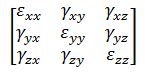
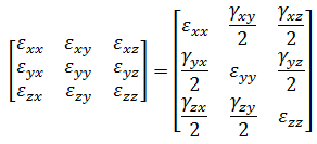
Tensor Displays a component of the strain in the chosen direction. For a static stress analysis with linear material models, the strains can be viewed in element, global, or cylindrical coordinates (just like the stresses).
Note: For MES analyses, Engineering strain results are available, not strain tensor results. The following matrix represents engineering strain (MES):
while tensor strain (Linear) is given by:
Beam and Truss The strain menu for beam and truss elements contains the following options.
- Axial Displays axial strain due to the load along the axis of the beam/truss. Tensile strain is considered positive.
- Bending about Axis 2 Displays extreme fiber strain due to moment about the 2 axis. This is valid only for beams. Tensile strain is considered positive.
- Bending about Axis 3 Displays extreme fiber strain due to moment about the 3 axis. This is valid only for beams. Tensile strain is considered positive.
- Worst Combination For beam elements, displays the worst combination of axial, bending about axis 2 and bending about axis 3. Mathematically,
  Worst = (sign of P/A)(ABS(P/A)+ABS(strain about axis 2)+ABS(strain about axis 3))
  
  For truss elements, the worst strain is equal to the axial strain (P/A).

Strain Energy Density

If this command is selected, the model will be shaded according to the strain energy density. The strain energy of an element is defined as the energy absorbed by the element due to the loading. This can be calculated on a per volume basis as:.

Normalized Stress and Strain

For the following linear analysis type:

Natural Frequency (Modal)

You can optionally output normalized stress and strain results. Do this by enabling the Normalized Stress and/or Normalized Strain option under the Output tab of the Analysis Parameters dialog box.

The sole purpose of these results is to show the relative stress and strain distribution within the model. That is, you can locate the regions of maximum or minimum stress and strain, but you cannot quantify the results using only a modal analysis. Since the results are not scaled to any specific excitation, the absolute stress and strain values have no meaning.

Autodesk Simulation Moldflow Results

Where applicable, Autodesk Simulation Mechanical models can be exported to Autodesk Simulation Moldflow Advisor or Insight to simulate the injection molding process. Once a Moldflow simulation has been completed, additional results will be available for visualization in the Results environment of Autodesk Simulation Mechanical. These results are chosen from within the Moldflow Result panel on the Results Contour tab of the ribbon. Among the Linear analysis types, the Moldflow results are available only for Static Stress with Linear Material Models. Moldflow results are also available for all Nonlinear structural analyses, except for Natural Frequency (Modal) with Nonlinear Materials. The following results are available:

The Residual Stress Tensor drop-down menu is used to select one of six residual stress tensor components (XX, YY, ZZ, XY, YZ, and ZX). These components are based on the in-cavity part stresses, at the completion of the molding process, from the Moldflow simulation. These are the stresses with the mold constraint still in place, and it is these residual stresses that cause a part to deform once it is released from the mold.
The CTE Tensor drop-down menu is used to select the Coefficient of Thermal Expansion tensor components in six directions (XX, YY, ZZ, XY, YZ, and ZX). These are the layer-based CTE results from the Moldflow analysis. All six CTE tensor components will not be available for all materials. Only materials with anisotropic thermal properties defined will have six CTE components.

Note: It is not necessary to run an Autodesk Simulation Mechanical analysis before exporting a model to Moldflow. However, you must at least execute the Check Model command. Likewise, it is not necessary to run an Autodesk Simulation Mechanical stress analysis to view the Moldflow results. You only have to enter the Results environment.

Element Displacements

The results under the Element Forces and Moments are primarily results for line elements: truss, gap, beam, boundary elements, and so on.

Stretch This command will color the gap, boundary, truss or spring elements based on the change in the length. For gap, truss and spring elements, a positive value indicates tension. For boundary elements, a positive value indicates the element is in compression.
Twist This command will color the boundary elements based on the element's rotation. The direction follows the right-hand rule directed from the elements attachment node to the free end.

Element Forces and Moments

The results under the Element Forces and Moments are primarily results for line elements: truss, gap, beam, boundary elements, and so on.

Axial Force Displays the axial force (local 1 direction) for all types of line elements: truss, beam, spring, gap, and boundary elements. For truss, spring, and gap elements, a positive value indicates tension, and a negative value indicates compression. For boundary elements, a positive value indicates the element is in compression, and a negative value indicates the element is in tension. For beam elements, see the paragraph Direction of Local Forces and Moments for Beam Elements below.
Shear Force in Axis 2 Displays the shear force in the local 2 direction for beam elements.
Shear Force in Axis 3 Displays the shear force in the local 3 direction for beam elements.
Torque Displays the torsion in a beam element (moment about the local 1 axis) and rotational boundary elements. For boundary elements, the direction of the torsion in the element at the node of attachment to the model follows the right-hand rule directed from the elements attachment node to the free end. For beam elements, see the paragraph Direction of Local Forces and Moments for Beam Elements below.
Moment About Axis 2 Displays the moment about the local 2 axis for beam elements.
Moment About Axis 3 Displays the moment about the local 3 axis for beam elements.
Plate Bending Moments When active, the bending moment tensor

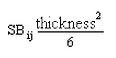
is used for all plate stress calculations. The bending moment tensor is a distributed moment (line moment, moment per unit length). The most easily interpreted results come from the Results Contours Stress Tensor. The mathematical calculations for von Mises, Tresca, maximum and minimum principal stresses are performed, but provide results equivalent to the bending stress values multiplied by

Direction of Local Forces and Moments for Beam Elements:

Component	Structural Beam
Local 1 Force	positive (+) value indicates tension, negative (-) value indicates compression.
Local 2 Force	Node i: positive value in direction of negative local 2 axis. Node j: positive value in direction of the positive local 2 axis.
Local 3 Force	Node i: positive value in direction of negative local 3 axis. Node j: positive value in direction of the positive local 3 axis.
Local 1 Moment	Node i: positive value in opposite direction from right-hand rule about local 1 axis (left-hand rule). Node j: positive value follows right-hand rule about local 1 axis.
Local 2 Moment	Node i: positive value in opposite direction from right-hand rule about local 2 axis (left-hand rule). Node j: positive value follows right-hand rule about local 2 axis.
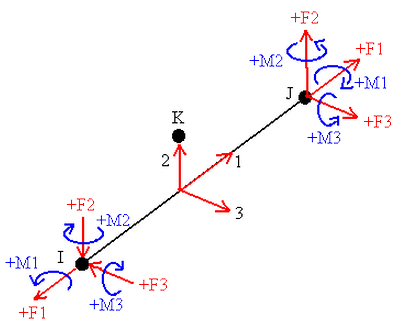
Local 3 Moment	Node i: positive value in opposite direction from right-hand rule about local 3 axis (left-hand rule). Node j: positive value follows right-hand rule about local 3 axis.

Figure 2: Direction of Local Forces and Moments for Beam Elements

Power Spectrum Density

When a random vibration analysis is performed and the option to output a power spectrum density is selected, the RESULTS will contain the item Power Spectrum Density. (See the page Setting Up and Performing the Analysis: Linear: Analysis Parameters: Random Vibration for activating the option.) The power spectrum density can be graphed as follows:

Display any type of result for the model, such as displacement or stress.
Select the node or nodes where a power spectrum density is appropriate, right-click, and choose Graph Value(s).
Once the graph is created, choose Results Inquire Graphs Power Spectrum Density to display one of the following results:
- X Displacement: display the power spectrum density of the X displacement.
- Y Displacement: display the power spectrum density of the Y displacement.
- Z Displacement: display the power spectrum density of the Z displacement.
- X Rotation: display the power spectrum density of the X rotation.
- Y Rotation: display the power spectrum density of the Y rotation.
- Z Rotation: display the power spectrum density of the Z rotation.

Keep in mind that the results are relative to the supports. They refer to power spectrum density with respect to the input excitation.

If multiple nodes were plotted, the power spectrum density needs to be activated for each node, one at a time. Right-click the node of interest in the browser and choose Set Active before attempting to display the power spectrum result. (See the page Results: Results Environment: Graphing the Results of an Analysis for general instructions.)

Reactions

This command displays the internal forces and reaction forces. The types of results to display are as follows:

Internal Forces In Linear, this menu displays the internal force reaction at each node. It is not the support reactions; use the Residual Forces command. You can either have the magnitude of the reaction force displayed or the individual components along the global axes.
Applied Forces Displays the force applied to each node. You can either have the magnitude of the applied force displayed or the individual components along the global axes.
Reaction Forces(Negative) Displays the residual force at each node (sum of applied and reaction). This is what most engineers consider to be the support reactions except that the residual force is the force of the model on the surroundings. The residual forces and support reactions are equal and opposite. You can either have the magnitude of the residual force displayed or the individual components along the global axes.
In MES/nonlinear, this menu displays the reaction forces at each node. The results are nonzero at boundary conditions, prescribed displacements, impact walls, and surface to surface contact.
Internal Moments In Linear, this menu displays the internal moment reaction at each node. It is not the support reactions; use the Residual Moment command. You can either have the magnitude of the reaction moment displayed or the individual components along the global axes.
Applied Moments Displays the moment applied at each node. You can either have the magnitude of the applied moment displayed or the individual components along the global axes.
Reaction Moments(Negative) Displays the residual moment at each node (sum of applied and reaction). This is what most engineers consider to be the support reactions except that the residual moment is the moment of the model on the surroundings. The residual moments and support reactions are equal and opposite. You can either have the magnitude of the residual force displayed or the individual components along the global axes.
In MES/nonlinear, this menu displays the reaction moments at each node. The results are nonzero at boundary conditions and prescribed rotations.

Each of the results type has the following options:

Magnitude: Shade the model based on the magnitude of the result.
X: Shade the model based on the X component of the result.
Y: Shade the model based on the Y component of the result.
Z: Shade the model based on the Z component of the result.
Vector Plot: Show the result as an arrow at each node. The length and color of the arrow represents the magnitude of the result, and the direction of the arrow represents the vector direction of the result.
Note: The reaction forces/moments and residual forces/moments will be nonzero at nodes connected by smart bonding. (These results are normally 0 at the boundary between parts.)

Von Mises Precision

Precision is a method of highlighting stepped changes in results from one element to the next. In an ideal model, the stress would change smoothly between adjacent element. In the process of discretizing the model with elements, there will always be some change in results from one element to the next. The results are not continuous.

In a stress model for example, elements with shared nodes predict stresses independently at the node, and therefore the independent stress calculations provide a precision estimate for the model based on the von Mises stress. The precision value at a given node is calculated as:

By definition, the precision will vary between 0 (best) and 0.5 (worst). Nodes that are not shared between two or more elements have only one stress estimate and therefore a precision index of 0.

Example 1:

If 200 is the maximum von Mises stress in the model, then the precision at the following nodes (with up to 3 elements attached to the node) are as follows:

Node#	von Mises Stress			PrecisionValue	Comment
Node#	Value 1	Value 2	Value 3	PrecisionValue	Comment
17	20	--	--	.0	Single element node
23	20	40	25	.05	.5(40-20)/200
36	150	120	200	.20	.5(200-120)/200

Example 2:

Given the following figure showing four elements surrounding node #5 and the following stresses:

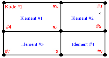
Element Number	Node Number	von Mises Stress
1	5	20,000
2	5	15,000
3	5	19,000
4	5	10,000

If the maximum stress in the model is 25,000 (at node 9 for example), the precision at node 5 is

precision node 5 = 0.5(20,000 - 10,000)/25,000 = 0.20

There is no guarantee that actual stresses will fall within the indicated range. The range in which they fall depends on how well the model is meshed, how well the actual part is modeled, and other factors. You should not consider differences smaller than the indicated precision significant. For example, if the precision is .1 and the maximum stress is 200, then differences of less than 20 stress units are not significant.

Applied Loads

Selecting this option will display the model with the input loads. Available loads for a structural analysis are temperature and voltage.

For Linear Stress,
1. The Results Contours Other Results Applied Loads Temperature is always available.
2. The contour is shown for all types of temperature loading specified in the Analysis Parameters from the model file, steady state heat transfer, or transient heat transfer.
3. The effect that the temperature has on the analysis also depends on the stress free reference temperature and the thermal multiplier. These contributions are not shown in the temperature contour.
For Mechanical Event Simulation/nonlinear stress,
1. The Results Contours Other Results Applied Loads Temperature is only available if a Source of nodal temperature has been assigned to the model in the Analysis Parameters.
2. The contour is shown for temperature loading from model file only. Temperature contours from steady state and transient heat transfer analyses are not available for plotting.
3. The effect that the temperature has also depends on the stress free reference temperature and the load curve multiplier. The effect of the load curve multiplier is shown by the temperature contour.

Element Properties

This commands will shade the model based on the shape of the elements. Most of the commands are applicable only to area and volume elements: 2D, plate, brick elements, and so on.

Each of the following options will shade the model based on the selected item.

Tip: Many of these options are used to shade the results of a solid mesh. Since the item of interest in this situation is inside the volume, it is recommended to activate the Display Options: Show Complete Mesh.

Volume If the Analysis Analysis Weight and Center-of-Gravity must be performed on the model, choosing the Results Contours Other Results Element Properties Volume command will display the volume of each element. The Weight and Center-of-Gravity calculator runs automatically if a weighted result summary is calculated in the Inquire: Results dialog.
Warp Angle The warpage of a quadrilateral (4-node) element or 4-node face of a solid element is displayed. There are three methods that can be used to calculate the warp angle.
- Minimum Fold Method or Maximum Fold Method If one of these commands are selected, the two quadrilateral fold angles are calculated and the minimum or maximum fold angle is used. The quadrilateral fold angle is obtained by dividing the quadrilateral into two triangles (adding one of two possible diagonals). The fold angle is the angle between the planar normals of these two triangles.
- Mid-Plane Method For this case, the sine of the mid-plane angle is equal to the height of any end node above the mid-plane divided by 1/2 the length of the shortest side. The mid-plane is the plane containing all 4 mid points of the edge lines. Each node is the same distance from this plane. The warp angle is calculated by multiplying the mid-plane angle by 2*square root of (2) so that it is comparable to the fold angle for squares bent at small angles. The factor of 2 results from using the angle from the mid-plane instead of the total fold angle. The factor of square root of (2) results from dividing by a half side instead of a half diagonal.

Node Angle If active, then elements are displayed based on the largest node (interior) angle of any of the faces of the element.
Aspect Ratio If active, then elements are displayed based on their aspect ratio.
For triangular elements, the aspect ratio is the longest side divided by the height of the triangle above that longest side. This ratio is multiplied by the square root of (3/4) so that an equilateral triangle has an aspect ratio of 1.0.

For quadrilateral elements (plates and 2D), the aspect ratio is calculated in the following way: the length of the longest side is divided by the greatest distance from the longest side to another node of the quadrilateral. A square has an aspect ratio of 1.0. A rectangle with sides of 1 and 2 has an aspect ratio of 2.0.

For brick elements (8-node), the mid-points of the three pairs of opposite faces are connected to form three lines. These lines cross at the center of the brick and each pair of lines defines a plane. For each plane formed by two lines, the ratio of the distance from the plane to the endpoints of the third line, divided by half the length of the longest line forming the plane, is calculated. The aspect ratio for the brick is the largest of these three ratios. For rectangular solids, the aspect ratio is the same as the largest quadrilateral aspect ratio of any of the faces.

For wedge elements (6-node brick), a mid triangle is constructed using the mid points of the edge lines connecting the triangular faces of the wedge. Let b be the largest side of the mid triangle, h be the height of the mid triangle and hw be the length of the line between the mid points of the end triangles. The aspect ratio is the maximum of sqrt(3)*h/(2*b), hw/b and b/hw. A wedge element created by extruding an equilateral triangle a distance equal to the side has an aspect ratio of 1.0.

For pyramid elements (5-node brick), let h be the height of the point above the midplane of the quad. Let b be the longest midedge line of the quad, the aspect ratio is the maximum of the quad aspect ratio, h/b and b/h. A pyramid with a square base and a height equal to the base side has an aspect ratio of 1.0.

For tetrahedral elements (4-node brick), the height, hi, above the base triangle with area ai, is calculated for each of the 4 possible bases. The aspect ratio is the maximum of Cf * hi/sqrt(ai), sqrt(ai)/(Cf * hi) for all 4 base triangles. Cf is (3/4)^3/4 so that the aspect ratio of a tetrahedral with all sides equal is 1.0.

Long/Short Ratio If active, elements are displayed based on the long/short ratio. The long/short ratio is the ratio of the longest edge length divided by the shortest edge length.
Area to Volume Ratio If active, then solid elements are displayed based on the ratio of the area divided by the volume. Specifically, the area to volume ratio is defined by the square root of the (Area/6) divided by the cubed root of the Volume. A cube has an area to volume ratio of 1.0. Flat elements (plates) have an area to volume ratio of 1.0.
Thickness of plateThis command is only applicable to plate or shell elements. The contour will vary based on the thickness of these elements.
Tetrahedral Collapse Ratio This command is applicable to brick models that include 4-node tetrahedral elements. When chosen, tetrahedral elements are displayed based on the ratio of longest edge length in the element and the shortest height (L/h). Other element types are not shaded.
Tip: Since the complete mesh needs to be displayed to see the interior elements, and the number of tetrahedral elements is usually small compared to the other element types, it can be hard to see the results through all the other unshaded elements. Use the Filter Modules to select only the shaded elements, and then hide the unselected elements.

Element Length If activated, line elements (beam, truss, and so on) are displayed based on the length of each element. Other element types are not shaded.