Given: The bucket of the front-end loader consists of two identical mechanisms. Each mechanism carries a load of 12 kN (24 kN total for the front-end loader) as shown in the figure below. Include the live load and gravity in the analysis.
Find: A preliminary design with:
- the optimum cross sections for the three links AB, BCE, and DEFG, based on minimizing the weight of the structure and limiting the stress to 100 MPa
- the size required for cylinders CD and FH.
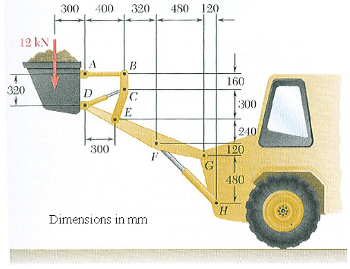 Figure 1 |
Since we are after a preliminary design and only considering in-plane effects, the shape of the cross-section is not overly important. Thus, beam elements with a rectangular cross section will be used. (Once the solution is found, a different shape with similar area and section modulus can be substituted, if needed.)
The optimization procedure is performed in the following basic steps:
- Part One – Build the Model. Create new model; draw and divide lines; and input loads, constraints, and parameters). Use a reasonable initial cross-section for the links.
- Part Two – Run the Analysis. This step will check the validity of the model and provide additional input for the optimization process.
- Part Three – Specify the Design Variables., These are the dimensions that will be changed to achieve the appropriate optimization goals.
- Part Four – Specify the Design Optimization Parameters.
- Part Five – Run the Design Optimization Analysis.
- Part Six – Review the Optimum Results.
You can create the geometry and input in either of two ways:
- Build the model yourself by following the steps on this page, beginning at Part One - Building the Model.
- Retrieve the archive of the model (front-end loader input.ach) located in the Models subfolder of the Autodesk Simulation installation directory (

 Archive Retrieve) and continue at
Part Two
– Run the Analysis.
Archive Retrieve) and continue at
Part Two
– Run the Analysis.
Part One – Build the Model:
The model will be created with beam elements for the arms (since they need to resist bending) and truss elements for the cylinder (since they will only transmit an axial force). The initial sections are as follows:
| Link | Part Number | Surface Number | Element Type | Initial Cross Section | Material |
|---|---|---|---|---|---|
|
width out-of-plane (b) x height in-plane (h) |
|||||
| DEFG | 1 | 2 | Beam | 24 x 250 mm | AISI 1005 Steel |
| Bucket | 2 | 3 | Beam |
rigid but small area |
AISI 1005 Steel |
| AB | 3 | 2 | Beam | 14 x 150 mm | AISI 1005 Steel |
| BCE | 4 | 3 | Beam | 20 x 150 mm | AISI 1005 Steel |
| CD and FH | 5 | any | Truss |
1900 mm 2 |
AISI 1020 Steel, cold rolled |
| Table 1: FEA Properties | |||||
Different part numbers will be used as a convenience for displaying or hiding each link in the Results environment. To simulate the pinned connections between the beams, end releases will be used on the bucket (at points A and D) and link BCE (at points B and E).
The model is planned as in Figure 2. The orientation of the model can be in any direction since beam elements are three dimensional, but let's use the XZ orientation of the model shown in Figure 2. (This makes the Front view natural.) The different part numbers are shown (P) based on the above table.
For beam elements, the orientation of axis 2 needs to be decided to enter the cross sectional properties. The desired orientation scheme is as follows:
- Axis 2 (weak axis of bending) lies in the plane of the model
- Axis 3 (strong axis of bending) points out of the model plane (parallel to the global Y-axis).
Since the orientation of beam elements is controlled by the surface number of the lines, this dictates the surface numbers (S), shown in Table 1 and in Figure 2. (See the paragraph Beam Element Orientation on the page Setting Up and Performing the Analysis: Analysis-Specific Information: Linear: Element Types and Parameters: Beam Elements for details on orienting beam elements.)
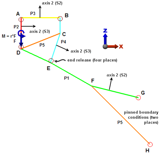 Figure 2: The FEA Model |
| Part numbers (P), axis 2 orientation decided by the user, and surface numbers (S) dictated by the orientation, are added to the figure. |
Draw the Geometry:
- Start a new FEA model ( New) and
- Set the analysis type to Linear: Static Stress with Linear Material Models.
- Click the Override Default Units button.
Since the dimensions are given in millimeters and the load in Newtons, lets choose units of Newtons, millimeters, and seconds for the model...
- Set the Unit System drop-down to Custom.
- Set the corresponding units of Force, Length, and Time to N, mm, and s, respectively.
- Click the OK button to set the units.
- Click the New button and enter a model name.
- Start drawing the mechanism at point G. Add a line using Draw Draw Line.
- Remove the check from the Use as Construction check box.
- Set the Part number and Surface number to 1 and 2, respectively, per Figure 2.
- Start the line at (0,0,0), and then activate the Use Relative check box. Per Figure 1, put the next points at the following relative positions. (To enter a coordinate, put the cursor in the X, Y, or Z box (or DX, DY, DZ), type the value, and press the Enter key.)
Point Relative Distance From Previous Point F (-480,0,120) E (-420,0,240) D (-300,0,140) Table 2 Keep the Define Geometry dialog box open. We will be creating additional lines.
- The lines may be off of the screen at this point. Use View Navigate Orientation Front View to re-orient the model view and to fit it to the display area.
- On the add line dialog, set the Part number and Surface number to 2 and 3, respectively, per Figure 2.
- Enter the next point A at a relative coordinate of (0,0,320).
- Set the Part number and Surface number to 3 and 2, respectively, per Figure 2.
- Enter the next point B at a relative coordinate of (400,0,0).
- Set the Part number and Surface number to 4 and 3, respectively, per Figure 2.
- Enter the next point C at a relative coordinate of (0,0,-160).
- The final segment of link BCE can be snapped to point E using the mouse. (The cursor will change to a padlock when the mouse is near point E, and clicking will snap the line segment to the point.)
- Click the X button to close the Define Geometry dialog box.
- Use View Navigate Enclose to show the entire model. Tip:
- If you used the wrong part or surface number when drawing the lines, simply select the line segment (Selection Select Lines), right-click, and choose Edit Attributes. Then set the correct part or surface number.
- If you enter a wrong dimension, you can undo the lines (on the Quick Access toolbar, click Undo), or select the wrong lines, delete them, and redraw the lines.
- If you used the wrong part or surface number when drawing the lines, simply select the line segment (Selection
- Beam elements should be divided into multiple segments to get a stress distribution along the length of the member. Therefore, select all of the lines (Selection Select Lines, then Selection Select All).
- Use Draw Modify Divide to split the selected lines into 4 lines each.
- Click the OK button to perform the divide operation.
- Use Draw
- Draw the lines representing the two cylinders using Draw Draw Line.
- Change the Part number to 5.
- Activate the Single Line option, since the two cylinders are not connected together.
- Use the mouse to draw a line from D to C.
- Use the mouse to start the next line at point F.
- Enter the final point at a relative distance of (600,0,-600).
- This completes the geometry, so click the X button to close the Define Geometry dialog box.
- Use View Navigate Enclose, if necessary, to show the entire model.
Specify the FEA Parameters:
- Enter a name for each of the parts. Select the Part <Unnamed> entry in the browser (tree view), right-click, and choose Rename. Type in the name of each link, per Table 1.
- Set the element type for each part per Table 1. Select the Element Type <Unknown> entry in the browser, right-click, and choose the appropriate element type. The element type for parts 1 through 4 can be set simultaneously by holding the Ctrl key and selecting each entry, then right-clicking on one of the selected entries.
- Set the element definition for each part per Table 1. Select the Element Definition entry in the browser, right-click, and choose Edit Element Definition. For the beam elements, highlight a cell in the Sectional Properties spreadsheet; this will enable the Cross-Section Libraries button. When the button is clicked, the Cross-Section Libraries dialog will appear. Set the Section database pull-down on the left to User Defined, and set the pull-down on the right to Rectangular. Based on the dimensions in Table 1 and the orientation of the beam elements, enter the height dimension for h and the width dimension for b. After entering the dimensions, click OK and OK to set the element definition. For the bucket (part 2), make the part rigid but with a small cross-sectional area. (The reason for a small area will be apparent when we do the design optimization.) In the analysis, the bucket will experience compression due to the 12000 N load and bending due to the moment. It will not experience any torsion. So, simply enter an area of 10 and moments of inertia I2 and I3 values of 100E6 in the Sectional Properties spreadsheet. Set the section modulus S2 and S3 to 0 so that no bending stresses will be calculated for the bucket. (The area is estimated from the load, length, and modulus of the bucket part to keep a reasonable deflection, and the inertia is a few times larger than the other cross sections.)
- Set the material properties for each part per Table 1. Select the Material <Unnamed> entry in the browser, right-click, and choose Edit Material. Parts 1 through 4 can be set simultaneously by holding the Ctrl key and selecting each entry, then right-click one of the entries. (Since the cross-sectional area of the bucket is small compared to the other sections, the bucket will be virtually weightless even though the material includes a mass density. If you truly wanted to make the weight 0, you can edit the Material for part 2 and set the mass density to 0.)
- Apply the constraints. Select points G and H (Selection Select Vertices, click point G, hold the Shift key, and click point H).
- Right-click in the display area and choose Add Nodal General Constraint.
- Click the No Translation button.
- Click the OK button.
- Right-click in the display area and choose Add
- The above constraints do not create a statically stable 3D model; the model is free to rotate about the Z axis. Add one more constraint by selecting the vertex where the load will be applied, right-click, and choose Add Nodal General Constraint.
- Activate the Ty check box and click OK. This condition will prevent the out-of-plane rotation.
- With the same vertex selected, right-click and choose Add Nodal Force.
- Enter a Magnitude of -12000.
- Set the direction to Z.
- Click the OK button to apply the force.
- With the same vertex selected, right-click and choose Add Nodal Moment.
- Enter -12000*300 in the Magnitude field. The product will be calculated and
- Set the direction to Y. Note that the equation in the Magnitude field is evaluated as soon as you click the direction radio button and 3600000 appears in this field.
- Click the OK button to apply the moment.
- Apply gravity to the model. Click Setup Loads Gravity.
- Click the Set for standard gravity button and confirm that the direction is correct (Z multiplier is set to -1).
- Go to the Gravity/Acceleration tab and set the Accel/Gravity multiplier to 1.
- By default, the connection between beam elements is a rigid connection. Therefore, end releases need to be added at points A, B, D, and E to simulate the pinned condition. Based on the chosen orientation, we know that the moment about axis 3 (R3) needs to be released, but we do not know a priori whether to release the moment on the I end or the J end of the element. This can be determined by displaying the beam orientation marks (View Visibility Object Visibility Element Axis 1 and Element Axis 2). This shows us that R3 needs to be released on the I end of the beams at points D and B, and the J end of the beams at points A and E. (See Figure 3.) So,
- Select the beam element in the bucket at point D and in link BCE at point B (Selection Select Lines, click the first line, hold the Shift key and click the second line),
- Right-click and choose Add Beam End Releases.
- Activate the R3 check box for the I Node.
- Click the OK button to apply the end release.
- Repeat the process for the elements at points A and E and activate the R3 check box for the J Node.
- When done properly, the end release symbol will appear on the proper end of each beam element as shown in Figure 3.
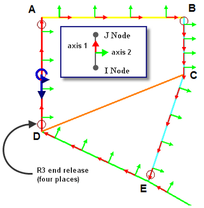
Figure 3: View Beam Orientations to set the Proper End Releases
The orientation marks at the center of each element show which direction is axis 1, and this determines which node is I and which is J. (Axis 1 runs from node I to node J.)
- Select the beam element in the bucket at point D and in link BCE at point B (Selection
- The beam orientation marks can be turned off (View Visibility Object Visibility Element Axis 1 and Element Axis 2).
Part Two – Run the Analysis:
In most cases, the input for design optimization is based on the results of the model as setup. In any event, it is always a good idea to perform the analysis first to make sure it runs properly before doing a more lengthy design optimization analysis. (This model is small enough that a Check Model is not really needed. Check the setup after performing the analysis.)
- Analysis Analysis Run Simulation.
- When it completes and the model appears in the Results environment, the first thing to check is the beam orientation to confirm that the weak axis of bending (axis 2 in our setup) and strong axis are oriented as intended. Select parts 1, 3, and 4 in the browser, right-click, and choose 3D Visualization. The rectangular cross section is shown for each element. Use View Navigate Orbit to rotate the model around. If the beams are oriented properly, the height of the rectangle should be in the XZ plane and the narrower width in the Y direction. Turn the visualization off when finished.
- Use Results Contours Displacement Displacement Magnitude to check the deflections. The maximum deflection of 3 mm is acceptable.
- Use Results Contours Stress Beam and Truss Worst to check the stress. The artificial stress in the bucket produces a large compressive stress which is not of interest. Right-click part 2 in the browser and clear Visibility. The stress in the remaining parts range from 51 N/mm
2
(51 MPa) compression to 60 N/mm
2
(60 MPa) tension. With the limit of 100 MPa, there is considerable room to reduce the cross section.
- One last thing to confirm: that the end releases are on the proper end of the elements to create the pinned connection at points A, B, D, and E. View the moment about the strong axis of bending (Results Contours Other Results Element Forces Moment About Axis 3). To check the moment on the fly, use Results Inquire Probes Probe. As you hold the mouse near a node, the results at that node are displayed. Confirm that the results near points A, B, D, and E are 0. (At node E, there should be a 0 moment in link BCE, and a large bending moment in link DEFG.)
Part Three – Specify the Design Variables:
The parameters that are adjusted by the design optimization are known as the design variables, and these are specified in the Element Definition dialog. Let's optimize the height of the cross sections for the links indicated in the problem statement.
- Return to the FEA Editor (Tools Environments FEA Editor).
- Right-click the Element Definition heading of part 1 in the browser and choose Edit Element Definition. Highlight a cell in the Sectional Properties spreadsheet, then click the Cross-Section Libraries button. Right-click in the h field and choose Set as Design Variable. The DV symbol appears to show that the height of the rectangular cross section will be a design variable. Click OK and OK to save the input.
- Repeat the above step for parts 3 and 4.
Part Four – Specify the Design Optimization Parameters:
- Use Analysis Analysis Optimization to access the Design Optimization dialog. The Design Variable tab shows the design variables set in the model. The Current Value column is filled in with the dimension entered in the Element Definition. For each of the design variables, enter a Lower Limit of 50; we do not want the cross section to be unreasonably small. Since the stress is below the allowable, there is no need to allow a larger upper limit, so enter an Upper Limit equal to the current value.
- The Performance tab is where the objective of the analysis and any constraints are entered. In this example, we want to minimize the weight (which generally minimizes the cost) and limit the stress. Click the Add Row button. By default, this adds an objective of minimizing the volume, which is equivalent to minimizing the weight. (Objectives are the quantities being minimized or maximized.)
- Since only one objective row can be specified, the Part to be minimized must be 0 or All. Tip: Design optimization adjusts the dimensions that are specified as design variables. Decreasing any part dimension reduces the volume of that part, which in turn reduces the total volume for the assembly.
- To get the input for the Current Value, switch back to the Autodesk Simulation Mechanical or Multiphysics interface and run the Analysis Analysis Weight and Center-of-Gravity command. This gives the total volume as 1.256e7.
- Enter 1.256e7 in the Current Value column of the Design Optimization dialog box.
Tip: Previously, the specified cross-sectional area of the bucket (part 2) was kept small, even though we wanted the bucket to be rigid. The purpose of using a small area is so that its volume would be small compared to the volume being optimized. If the volume of the bucket were to be very large relative to the other parts of the model, then a small change in volume of parts 1, 3, or 4 might represent an insignificant change in the total volume. We want to avoid this potentially misleading result. - The Limit Value of the volume can be estimated from the Weight and Center of Gravity dialog by scaling the volume of each part by the ratio of the design variable's Lower Limit/Current Value and summing the result. This yields a total minimum volume of the model of 4.7616E6. Enter this value into the Limit Value column.
- Since only one objective row can be specified, the Part to be minimized must be 0 or All.
- Click Close on the Weight and Center of Gravity dialog.
- Back in the Design Optimization dialog, Performance tab, click the Add Row button three times to add three new constraints. We want to set an upper limit on the stress for each part that is being optimized.
- Change the Objective/Constraint to Max Stress.
- Set the Type to Upper Limit.
- Change the Part numbers to 1, 3, and 4 respectively.
- The Current Value for each part can be found from the Results environment in the Autodesk Simulation Mechanical or Multiphysics interface. (Click the Results tab.) Display each of the three parts individually to determine the current stress for each (select the parts to hide in the browser, right-click, and clear Visibility).
- With the Results Contours Stress Beam and Truss Worst result shown for one part, the current value of stress for the current cross-section can be obtained. (Be sure to use the largest absolute value. The maximum stress can be negative or positive.)
- Clear the Visibility of this part and select Visibility of the next part. Repeat until you have determined the stress for parts 1, 3, and 4.
- With the Results Contours
- The Limit Value of 100 (MPa) maximum stress is per the problem statement, and the Current Value of the part stresses were determined in the preceding step. Enter these values, each in the appropriate row and column. The correct values are listed in Table 3 below.
Objective/ Constraint Loadcase Type Part Current Value Limit Value Volume All Minimize All 1.256E7 4.7616E6 Max Stress All Upper Limit 1 59.86 100 Max Stress All Upper Limit 3 5.42 100 Max Stress All Upper Limit 4 27.38 100 Table 3: Performance Tab Input
- The default input on the Parameters tab will be used, and the results checked to confirm that they were acceptable.
Part Four – Run the Design Optimization Analysis:
- Go to Analysis Perform Design Optimization.
- When the dialog appears, click the Analyze button to begin the optimization process.
- When the analysis completes, check the last lines of information in the display window (the optimization log file). The critical items are described in Table 4.
01 ** The change of constraints are less than limit! 02 ** Finished Optimization after 5 Iterations 03 ** Optimum Design Variables ** 04 =========================================================================== 05 Design Current Value Lower Limit Start Value Upper Limit 06 --------------------------------------------------------------------------- 07 1 1.8922e+002 5.0000e+001 2.5000e+002 2.5000e+002 08 2 5.0000e+001 5.0000e+001 1.5000e+002 1.5000e+002 09 3 7.6111e+001 5.0000e+001 1.5000e+002 1.5000e+002 10 =========================================================================== 11 ** Optimum Objective/Constraint Value ** 12 =========================================================================== 13 Obj/Const Current Value Limit Value Change/Violation 14 --------------------------------------------------------------------------- 15 Objective 9.38600e+006 1.25600e+007 25.270701 % Decreased 16 1st Const 9.96355e+001 1.00000e+002 -0.364452 % Not Violated 17 2nd Const 1.62569e+001 1.00000e+002 -83.743147 % Not Violated 18 3rd Const 9.99214e+001 1.00000e+002 -0.078580 % Not Violated 19 =========================================================================== 20 ** Finished Optimization !! ** Table 4: The Last Iteration of Design Optimization Analysis Line numbers were added to help with the following description. The analysis has converged (line 01) because the change in the user-entered constraints from one iteration to the next was less than the user-entered tolerance, and this was reached in fewer iterations than the entered maximum number of iterations (line 02). Line 15 shows the objective (volume, being minimized). The Change/Violation column indicates the optimum design is 25.3% less than the user-entered current value. The first constraint (line 16, stress) had an upper limit of 100 MPa specified. The final optimum value was 99.6 MPa. The second constraint (line 17, stress) was greatly under upper limit of 100 MPa. The stress is not higher because the design variable (the height of the cross section, line 08) is at the lower limit of 50 mm; thus, the cross section cannot be any smaller, so the stress cannot be any higher than 16.3 MPa. The third constraint (line 18, stress) is also at the limit of 100 MPa. (Text shown in bold is highlighted to correspond with this description.) - Click the Done button to close the analysis window. Since the results are acceptable, no changes are required. If the outcome were not acceptable, such as one of the constraints had been violated, then the design optimization could be re-run with different upper and lower limits on the constraints (Design Variable tab) or with different optimization parameters (Parameters tab).
Part Six – Review the Optimum Results
- From the Design Optimization Results menu, choose Design Optimization History. Then the Results frame contains each objective, constraint, and design variable in the drop-down menu. Select each item to see a graph of how the value changed with each iteration.
- Use the Results menu and choose Optimum Result. This will start a new instance of Autodesk Simulation and load a copy of the original model but with the design variables set to the optimum value calculated by the design optimization.
- In the Autodesk Simulation interface, click the Results tab to view the optimum model results. Following the sequence of steps performed on the original model, we find that the displacement magnitude is slightly higher (4.5 mm) than before, but still acceptable. Naturally, the stress results are acceptable. Thus, the answers to item 1 of the problem description are summarized in the following table.
Link Part Number Optimum Cross Section width out-of-plane ("b")
x height in-plane ("h")
DEFG 1 24 x 189 mm AB 3 14 x 50 mm BCE 4 20 x 76 mm Table 5: Optimum Cross Section - To get the cylinder sizes (item 2 of the problem description), hide all parts except for part 5. (Select parts 1 through 4 in the browser, right-click one of them, and clear Visibility.)
- Set the results type to Results Contours Other Results Element Forces Axial Force.
- The forces in the cylinders are as follows, determined either from the legend or by inquiring on the elements (Results Inquire Probes Probe).
Cylinder Axial Force CD 21400 N FH 72450 N Table 6: Cylinder Forces (to 4 Significant Figures) The size of the cylinders can be calculated based on an assumed fluid pressure.
Two archives of the model and results are located in the Models subfolder of the Autodesk Simulation Mechanical or Multiphysics installation directory:
- front-end loader input results.ach is the original model with the design variables defined
- front-end loader_OPT.ach is the model with geometry based on the optimum results.
This example is based on example 6.149 from Beer, Ferdinand P. and Johnston, E. Russell, Vector Mechanics for Engineers, Statics and Dynamics, McGraw Hill, 7th Edition, page 341.