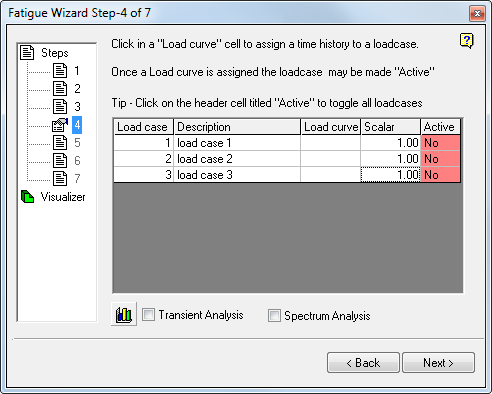
In step 4, define the cyclic loading, which is used later in the fatigue analysis.
The FE model is previously solved, and has linear static stress results for either a single or multiple load cases.
To define a cyclic event and a fatigue calculation, the analyst must assign a ‘load history’ to each of these load cases. The load history describes how the stresses calculated in the static FE model vary with time. In Fatigue Wizard, you can scale and combine any one or more of the load cases by a ‘load history’ to create the final cyclic stresses.
Fatigue Wizard automatically reads in the results for all load cases analyzed in the FE model. Use the methods described in the following sections to turn load cases on and off, define individual load curves to load cases, and define scalar multipliers for each load case.
This step takes the results of your analysis and multiplies them by Load History curves. These curves define the Fatigue Event.
For example:
You performed a Linear Static Stress analysis on your FE model.
This step takes the results of your analysis and multiplies them by a Load History curve. This curve defines the Fatigue Event.
For example:
Single Load Analysis
You performed a Linear Static Analysis using the loading shown in the following image, and reviewed your stresses.
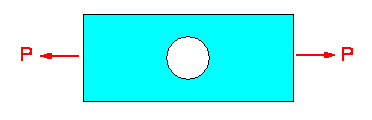
The load P is a static constant load.
But, in reality this load can be applied and then removed many times, as in the following image. If necessary, evaluate the fatigue performance of your model under this cyclic event.
For example:
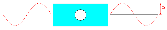
Or
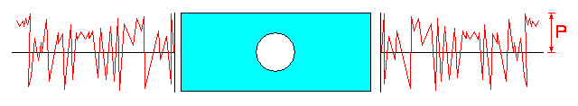
It is easy to create these conditions with Fatigue Wizard.
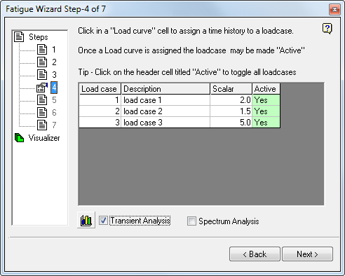
The following steps describe how to apply a load history to the static event. Click the "Load curve" field for the required load case from your Linear Static Analysis. For example, to define a load curve for Load case 3, click in the third row of the "Load curve" column.
This form displays, where you can input load curve data by various means.
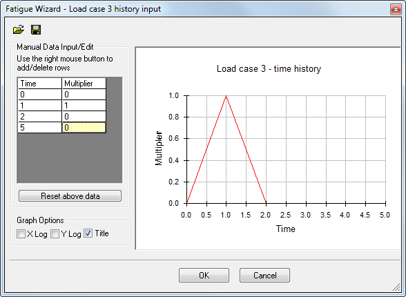
Method 1 is to enter load curve data into the form directly. To add or delete rows from the Time vs. Multiplier table, right-click and choose the desired command.
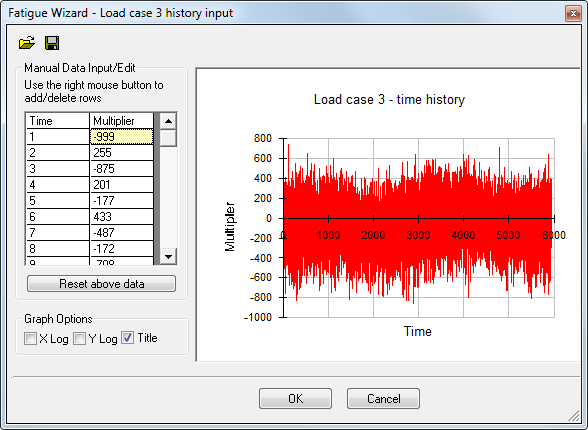
The second input method is to import a *.CSV file (comma-separated values). Several curves are included with the program installation. These curves (*.CSV files) are located within the \Addins\Fatigue Wizard subfolder of the Simulation Mechanical installation folder (typically C:\Program Files\Autodesk\Simulation 20xx ).
The following example illustrates an imported CSV file ("SAE test data bracket.csv" from the ...\Addins\Fatigue Wizard folder):
When the load curve data is entered or imported into the form and accepted, you are returned to the main 'Step 4' form. The form is updated to indicate that load curve data has been entered and assigned to a load case. In this case, the load curve for Load case 3 is "Defined" and "Active."
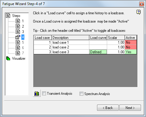
If necessary, after the load curve data is defined for a load case, you can remove it from the fatigue calculation by 'de-activating' the load case. Click the "Active" cell to toggle its status.
You can scale the load curve data. Enter a multiplier (set as 1.00 by default) in the "Scalar" cells.
Important notes on Load curves:
The load curves defined previously are MULTIPLIERS to your Linear Stress results for each active load case. Consider the following examples:
The Fatigue Stress used in calculations = Linear Static Stress x Load curve Multiplier.
For example, if the loading applied to your Linear Stress model represents a maximum load of 100N (for example) and your fatigue analysis load curve has a maximum value = 1.5. Then...
The Fatigue Stress used in the fatigue calculations = 100N x 1.5 = 150N.
You could also apply a load of 1N to your Linear Static model and then define your fatigue load curve to have a maximum value of 150.
Fatigue Stress used in calculations = 1N x 100 = 100N.
which will produce the same end result. This "unit load" technique is a convenient way to work, and is a common way to apply fatigue loads.
Multiple Load cases
If more than one load case is solved in the analysis, you can use more than one of these load cases in the fatigue analysis. Two methods exist within Fatigue Wizard for utilizing more than one load case—load case superposition, and a transient method. For more details on the theory of each method, see "Theoretical Overview".
Load Case Superposition
If more than one load is applied to the model simultaneously, you can assign separate load histories to each load case, and perform the necessary stress scaling and superposition.
Follow the steps described previously for each of the load cases required in the fatigue analysis. Load histories applied to each load case do not have to have the same number of points, but must all start and finish at the same value of ‘time’. If not, Fatigue Wizard warns you.
After you assign load histories to each load case, you can assign a multiplier to each load case. You can turn on or off the individual load cases by clicking in the ‘active’ cell.
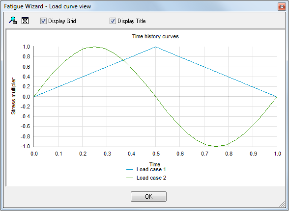
To view all load cases on a single graph, press the "View all load curves" button (  ). In the view that displays, ensure that all curves start and end at the same times.
Transient Analysis
A transient analysis differs from the superposition method in that no load histories are applied to the individual load cases. Instead, Fatigue Wizard takes the results from various load cases within a Linear Static Analysis and uses them to define the sequence of stress.
The stress history that constitutes the fatigue cycle is made up of the individual stress states sequenced one after another. No load case superposition is necessary.
To enter transient information, select the load cases to define your cycle, enter a stress scale factor (if necessary), and activate the Transient Analysis checkbox. The Load curve column is hidden while in Transient Analysis mode.
The order of the stress states in the cycle is determined by the order in which they appear in the FE model. Therefore, if using the transient method, set up the FE model correctly for the anticipated fatigue analysis cycle.
Spectrum AnalysisA spectrum analysis is a simple extension of the previously described transient analysis. In the same way, the spectrum analysis does not perform any load case superposition. Stress histories are created within Fatigue Wizard from sequences defined from individual load cases. Fatigue Wizard takes the results from various load cases within a Linear Static Analysis and uses them to define the sequence of stress.
The spectrum analysis differs from the simple transient analysis in that an additional text file is used to define multiple sequences of stresses. The text file is used to define both the sequence of stress (constituting a single stress history), and a number of repetitions of this history.
Fatigue Wizard then performs a damage summation over all of the repetitions of each of the individual stress cycles defined by the spectrum file.
To set up a spectrum analysis, activate the Spectrum Analysis checkbox. Then you can click the standard file selection icon that appears to associate a spectrum file. The spectrum analysis takes the scale factors from the Step 4 dialog box, and those read from the spectrum file, to create multiple stress histories. Each of these discrete stress histories is used to calculate damage. Then this damage is all summed over the number of repetitions of the stress history, also defined within the spectrum file. A Total damage/Life is then reported over the entire spectrum.
The following example describes the process of performing a spectrum analysis:
Example spectrum file
The spectrum file begins as a spreadsheet (for example, in Microsoft Excel) and is then saved as a *.CSV file.| 5 | |||||
| 10000 | 5000 | 20000 | 100 | 10 | $ |
| 0 | -1 | 1 | 0 | 0 | $ |
| 0.05 | 1 | 0 | 2 | -5 | $ |
| 0 | -1 | 1 | 0 | 0 | $ |
- The first row of the spectrum file defines the number of load histories defined in the file (in the example there are 5)
- The file is then considered to be separated into the same number of columns as there are load histories.
- The top row of each of these columns defines the number of repetitions of this load history. In the example above, the load history defined by column 1 is repeated 10000 times, the load history of column 2 is repeated 5000 times, and the load history of column 3 is repeated 20000 times, and so on.
- The remaining rows of each of the columns are multipliers of the stresses for each of the load cases in the FEA. (Note: These multipliers are applied in addition to multipliers specified on the main Step 4 form!)
- The multipliers in each column are used to define the multiple load histories, which constitute the overall load spectrum. In the previous example, there are three discrete load histories to make up the complete spectrum.
- A damage calculation is then performed for each individual load history and multiplied by the number of repetitions defined. This process is repeated for each load history, and the damage summed over all load histories to give a total life.
- The order of the stress states in the cycle is determined by the order they appear in the FE model. Therefore, if using the spectrum method, set up the FE model correctly for the subsequent fatigue analysis.
- A more detailed description of the spectrum file is contained in "File Formats: Spectrum File".