A German engineer, Albert, carried out the first known fatigue investigations in the early 19th century. It had been understood that a material subjected to repeated loading would eventually fail. However, it was the widespread failure of railway carriage axles after many miles of apparently faultless service which began to draw attention to the phenomenon that later became known as fatigue.
Most engineering components or structures experience some form of cyclic loading. Failure in such components typically means the initiation of small cracks, which eventually link to form large cracks and catastrophic failure. The crack initiation begin at stress levels well below the monotonic yield stress of the material. Over time, (repeated) damage accumulates until eventual failure. It has been widely suggested that over 90% of structural failures occur as a result of fatigue damage.
Two basic approaches are available to estimate the number of repeats of a cyclic load a material or component can withstand.
The early methods utilized material data first collated in the 19th century by Wholer. This technique related the stress in a component to an empirical curve, known as the S-N curve, (or Wholer line) to obtain an estimate of the number of cycles to failure. This technique is still used today and is commonly known as the stress-life approach. This technique uses the component stress and makes the assumption that the stress remains in the elastic region of the material. Therefore, it is best suited for fatigue failure where 100000+ cycles are required for failure.
The second and more modern technique utilizes the material strain to predict failure. Curves relating strain to cycles can be prepared from test or empirical formulae similar to those used for the stress-life approach. The major benefit in using this technique is that the strain-life curve represents the local Strain State of the component, and can account for local plastic deformation. This greatly increases the accuracy of the life prediction at loading levels where local yielding occurs.
Fatigue Wizard uses both techniques to predict fatigue life.
Definition of Loading
Fatigue damage is caused by loading a structure with repeating loads over a period of time. To analyze fatigue failure it is necessary to define the applied load. in the Fatigue Wizard, you can define two basic loading types, the simplest form being the constant amplitude harmonic.
This loading is fully described by the definition of a stress amplitude sa and a mean stress sm. The repeating cycle is a single harmonic period, that is points 1-2-3-4 in Figure 1.
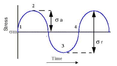
Figure 1 Constant Amplitude Harmonic Loading
The second type of loading, and a more general case, is the variable amplitude load.
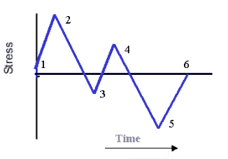
Figure 2 Variable Amplitude Loading
Variable amplitude loading is made up of many individual constant amplitude cycles. These individual cycles can each have different amplitude and mean and can be superimposed or subsequent. Figure 2 shows a simple example of a variable amplitude load. You can see that there are two simple cycles: 1-2-5-6 forms a large amplitude single cycle onto which the smaller cycle 3-4-3 is superimposed. A variable amplitude loading can therefore be broken down into a number of simpler constant amplitude loads. Then they are used in the fatigue analysis to predict damage.
If a variable amplitude load is to be used for fatigue calculation, a method must be applied to extract the ‘sub-cycles’. Fatigue Wizard applies it by a standard rainflow counting algorithm.
Rainflow Counting and Fatigue Damage
Both the stress-life and strain-life techniques of predicting fatigue failure rely on a single cycle damage curve. This damage curve correlates number of repetitions with stress or strain amplitude for a single simple cycle. This curve can be used directly if the structural loading is the simple constant amplitude type. However, if a variable amplitude loading is defined, several steps need to be followed to calculate a life for the applied load.
First the load history is peak-valley picked. This process scans the time history for any points which are not ‘reversal’ points and discards them, thus reducing unnecessary data. Next the reduced time history is processed with a standard rainflow counting algorithm, which extracts individual single cycles. These single cycles are then used with the single cycle damage curves to calculate a life for each cycle.
After a life is calculated for each individual cycle in the time history, a method of determining the cumulative damage or total life is required. Fatigue Wizard utilizes the well-documented ‘Miners Rule’. This rule states that the total damage accumulated over a load history is the linear sum of the damage of individual cycles.

or

where N is life in repeats and D is the damage.
Stress Life Technique
The stress life technique utilizes a single cycle damage curve known as the SN curve. This curve relates stress amplitude to number of cycles to failure. Since this technique has been used widely for many years, such curves and material data relating to such curves are readily available. The stress value used with the curve depends on the data represented in the curve, and to an extent, the discretion of the engineer. The uniaxial version of Fatigue Wizard uses the ‘worst absolute principal’ stress in its calculations, since the direction of the stresses is assumed constant.
Fatigue Wizard generates the SN curve internally from the material data input by the engineer. Data required are the monotonic tensile strength of the material, and an ‘endurance limit’.
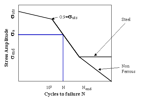
Figure 3 SN Curve
The SN curve takes the form shown in Figure 3. SN curves are always plotted on log-log scales, as shown. The curve starts from the monotonic tensile strength suts at log(N)=1. It is then common to approximate the range up to a value of 1000 cycles by a straight line to a value of 90% of suts. The main slope of the SN curve extends from the 1000 cycle point to a life value corresponding to the ‘endurance limit’ and a stress amplitude equivalent to send. The behavior beyond the endurance limit then depends on whether the material is a ferrous alloy or non-ferrous alloy. It is typical for steels to show a real endurance limit and a flattening of the SN curve. Conversely, aluminium alloys and other non-ferrous alloys show a less distinct flattening of the SN curve at high cycles. Fatigue Wizard allows the user to distinguish between these two cases.
Mean Stress Effects
You usually present SN curves for a fully reversed test. This means that the stresses applied cycle between equal tensile and compressive states. In realistic structural loading, it is more common for the cyclic loads to oscillate around a non-zero mean state. This non-zero mean state has a significant effect on the life to failure. A method is required to account for the presence of a mean stress in the cycle when using the standard SN data.
Fatigue Wizard allows you to calculate the fatigue life using ‘no-mean’, ‘Gerber’ and ‘Goodman’ corrections.
Stress Concentration
It is usual for FE analyses to explicitly model and calculate stresses in areas of local concentration, so any scaling of nominal stress is unlikely to be required. However, should any linear scaling of the calculated FE stresses be required Fatigue Wizard provides a general scaling factor Kt.
se = Kt.snominal
Where se = scaled elastic stress
Endurance Limit Modifiers
SN curve data is usually presented from tests on standard sized polished specimens. Applying this ‘laboratory’ test data to real engineering components sometimes requires some correction. The corrections usually take the form of ‘modifiers’ applied to the specimen endurance limit.
Modifiers can be applied to take account of size, surface finish, stress gradients, surface treatments, ‘loading type, and so on. These modifiers are well documented in many engineering texts and readily available to the engineer if required.
send-modified = send . nsize . nsurface …
where n is the appropriate modifier
Fatigue Wizard supplies standard modifiers for surface finish effects and statistical effects and a general modifier to input a calculated combined value. Fatigue Wizard modifies the SN curve by scaling the specimen endurance limit as above, and rotating the SN curve about the 1000 cycle point.
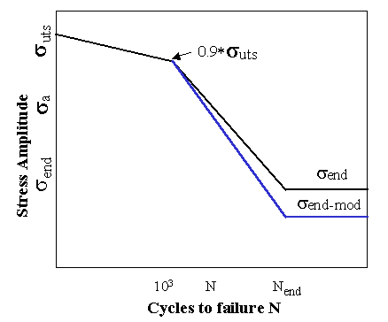
Figure 4
Strain Life Technique
The strain-life technique was developed in the 1960’s as an improvement to the stress-life technique for predicting fatigue failure in material, which undergoes plastic deformation. The principle is the same, in that strain amplitude (rather than stress) is measured or calculated, for a cyclic load, and compared to an empirical graph of strain amplitude against life. The advantage over the stress-life approach is that there is no inherent assumption in the test data regarding totally elastic deformation.
Strain-Life Curves
Strain-life curves describe the fatigue behavior of laboratory tested specimens. Specimens are usually tested under fully reversed strain controlled load and correlated against life to crack initiation. An empirical curve of strain amplitude against cycles to failure is plotted.
For low levels of strain where deformation is completely elastic, the fatigue behavior correlates to the stress amplitude and

Where sf’ is the fatigue strength coefficient and b is the fatigue strength exponent, both extracted from the log-log fit of stress amplitude against life.
For high levels of strain where deformation is predominantly plastic the fatigue behavior correlates best with strain amplitude such that

Where ef’ is the fatigue ductility coefficient and c is the fatigue ductility exponent, both extracted from the log-log fit of plastic strain amplitude against life.
The general strain life curve or Coffin-Manson curve is then described as a combination of these two individual straight line curves, such that

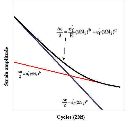
Figure 5 Constant Amplitude Strain Life Curve. Coffin-Manson relationship.
Approximate various Strain-Life coefficients that are not available
There are various methods to approximate strain based material data from the more readily available monotonic data, such as tensile strength, modulus, and so on. The method used by the Fatigue Wizard is the method used by Seeger/Beste. It is available in many texts on strain based fatigue calculation. This technique approximates the strain life curve (strain based coefficients) using the following formulae:
Steels:
- K' = 1.65 * UTS
- n' = 0.15
- Sf = 1.5 * UTS
- b= -0.087
- c= -0.58
- Ef = 0.59 (if UTS/E<0.003)
- Ef = 0.59*(1.375-125*UTS/E)
Others:
- K' = 1.61 * UTS
- n' = 0.11
- Sf = 1.67 * UTS
- b= -0.095
- c= -0.69
- Ef = 0.535
Mean Stress Correction
The constant amplitude life curve described previously is generated through material testing under fully reversed loading, that is, with zero mean shift. In realistic engineering loading cycles, it l inevitably exists with a non-zero mean strain.
To correct for the existence of non-zero means in the strain cycle, Fatigue Wizard uses two corrections to the simple strain life curve, namely the Morrow correction and the Smith-Watson-Topper correction.
Strain-Life curve with Morrow correction

Strain-Life curve with SWT correction

Elastic-Plastic Material Data
Since strain-life data is extracted from materials, which are subjected to cyclic loading beyond the elastic limits, it is necessary to define a cyclic stress-strain material curve.
Fatigue Wizard utilizes two well-documented empirical formulae for the definition of cyclically stable stress-strain curve.
The cyclic stress-strain curve is constructed by using the Ramberg-Osgood relation to determine material constants K’ and n’. That is, the cyclic hardening coefficient and the cyclic hardening exponent.
Ramberg-Osgood relationship

To generate a complete cyclic stress-strain curve, Masing’s Theory is used such that:

By combination of these two relationships a full hysteresis loop of the cyclically stable stress-strain curve can be generated from the two material constants.
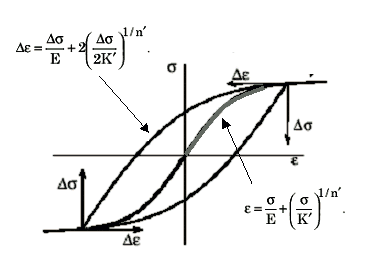
Figure 6 Cyclically stable Stress-Strain Curve
Neuber Correction
Many FE based fatigue codes use the results of elastic FE analyses. This enables you to carry out relatively simple FE calculations without incurring expense and time of running non-linear solutions. If a strain based life calculation is to be performed later using these elastic stresses, put a method in place for converting the FE based elastic stress to an equivalent elastic-plastic stress (and strain).
Of the many methods proposed for this conversion, Fatigue Wizard utilizes the most common, the Neuber correction.
Stress-Life Approach.
- Read elastic stress data from FE Results.
- Extract Worst Absolute Principal Stress.
- Scale Elastic Stresses by Kt.
- Extract Cycles from Time History of Load by Rainflow Counting.
- Modify SN Curve According To Endurance Limit Modifiers.
- Calculate Damage for Cycles With Mean Stress Correction.
- Sum Damage According To Linear Miners Rule.
- Output Fatigue Life or Safety Factor for all Nodes.
Strain-Life Approach
- Read elastic stress data from FE Results.
- Extract Worst Absolute Principal Stress.
- Scale Elastic Stresses by Kt.
- Carry out Neuber Correction To local stress.
- Construct complete local stress/strain time history using cyclically stable stress/strain curves.
- Extract all closed hystereses loops in time history.
- Construct Single Cycle Strain-Life Curve from Material Data.
- Modify Strain-Life curves according to endurance limit Modifiers.
- Calculate Damage for Cycles With Mean Stress Correction.
- Sum Damage According To Linear Miners Rule.
- Output Fatigue Life or Safety Factor for all Nodes.