Given: A stainless steel cylinder (AISI 304) initially at 600 K is quenched by submersion in an oil bath maintained at 300 K with a convection of h = 500 W/m 2 K. The length of the cylinder is 60 mm and the diameter is 80 mm. Material properties for stainless steel (AISI 304), taken from Introduction to Heat Transfer, are: density = 7900 kg/m 3 , conduction coefficient = 17.4 W/m K, and specific heat = 526 J/kg K.
Find: What are the temperatures at the center of the cylinder, at the center of a circular face, and at the mid-height of the side at three minutes into the cooling process?
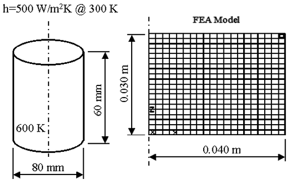
Figure 1: Problem Geometry
This example only covers setting up and performing the analysis. For instructions on building the model, see Creating the Cylinder with Convection Model. If you have not built the model, you can open the cylconv_input.ach file in the Models subfolder of the Autodesk Simulation installation directory.
Method 1: 2D Axisymmetric Model
- Right-click the Element Type heading for Part 1 in the tree view and select the 2D command.
- Right-click the Element Definition heading for Part 1 and select the Edit Element Definition command. Select the Axisymmetric option in the Geometry Type drop-down menu and click OK.
- Right-click the Material heading for Part 1 and select the Edit Material command. With [Customer Defined] highlighted, click Edit Properties. Type 7900 in the Mass Density field, type 17.4 in the Thermal conductivity field and type 526 in the Specific Heat field. Click OK twice.
- Click the + next to the Surfaces heading under Part 1 to display the two surfaces on this part. Right-click the Surface 2 heading and select the Add
 Surface Convection Load command. Type 500 in the Temperature Independent Convection Coefficient field and type 300 in the Ambient Temperature field. Leave the load curves set to 0 to indicate that the loads do not change with time. (Since the load does not follow a load curve, the Load Curve Magnitude value is not important.) Click OK.
 - Right-click the Analysis Type heading in the tree view and select the Edit Analysis Parameters command. The analysis must run for 180 seconds (3 minutes) per the problem statement. If a calculation time step of 1 second is used, then 180 steps must be calculated. Output every tenth step. Use this input: Initial Time is left as zero. On the first row of the Event spreadsheet, enter the Time as 180, the Steps as 180, and the Output interval as 10.
- Click the Options tab and type 600 in the Default nodal temperature field. Without changing this value, the model would start at 0 degrees at time 0.
- Click the Advanced tab. There are no nonlinear effects in the model (orthotropic conductivity or radiation), so type 0 in the Number of time steps between matrix reformulation field.
- Click OK to close the Analysis Parameters dialog box.
- Select Analysis Analysis Run Simulation to perform the analysis. During the analysis, the results are displayed in the Results environment as they are computed.
- To look at the results at a time of 180 seconds, use Results Contours Load Case Options Last Results.
- To read the actual values at the appropriate nodes, use Results Inquire Inquire Current Results. Click the bottom left node (the center of the cylinder) to read the value (403.4). Click the top left node (the center of the circular face) to read that value (371.0). Click the bottom right node (the midheight of the side) to read that value (362.7).
- A graph of the temperature results at any node can be created. Select the appropriate node, right-click, and select Graph Value(s).
Method 2: 3D Brick Model
The 3D model is created in a different Design Scenario by starting with a copy of the 2D model's Design Scenario. Due to symmetry, only a 90-degree segment of the entire 360 degree part will be modeled.
- Click the FEA Editor tab to return to the that environment.
- Right-click Design Scenario 1 and choose Copy. It creates a duplicate of the 2D mesh which is used to generate the 3D mesh.
- Select all of the lines in the model using Selection Select Lines and then Selection Select All.
- Revolve the 2D mesh to create the brick elements. Select Draw Pattern Rotate or Copy. Activate the Copy check box and type 10 in the adjacent field. Activate the Join check box.
- Type 90 in the Total angle field and select DZ. The rotation center point should be (0,0,0). Click OK to revolve the mesh and create a quarter cylinder. This can be confirmed by changing to the isometric view (View Navigate Orientation Isometric View).
- Right-click the Element Type heading for Part 1 in the tree view. Select the Brick command. All other input was copied from the 2D model so does not need to be changed.
- Select Analysis Analysis Run Simulation to perform the analysis. During the analysis, the results are displayed in the Results environment as they are computed.
- To look at the results at a time of 180 seconds, use the Results Contours Load Case Options Last Results command.
- To read the actual values at the appropriate nodes, select Results Inquire Inquire Current Results. Click the bottom node (the center of the cylinder) to read the value (403.0). Click the top node (the center of the circular face) to read that value (370.7). Click the bottom right node or bottom left node (the midheight of the side) to read that value (362.6).
Note: The node at the center of the circular face is tricky to select from the isometric view. You may need to switch views to get this node.
Comparison of Results
The following table presents results obtained from the analysis in Introduction to Heat Transfer and the two analyses performed with software.
An archive of the model cylconv.ach is located in the Models subdirectory of the Autodesk Simulation installation directory.
|
Temperature at 3 minutes (K) |
|||
|
Center of Cylinder |
Center of Top Circular Face |
Midheight of Side |
|
| Reference | 405 | 372 | 366 |
|
2D analysis |
403.4 | 371.0 | 362.7 |
|
3D analysis |
403.0 | 370.0 | 362.6 |
Reference
Introduction to Heat Transfer, Incropera, Frank and DeWitt, David, John Wiley & Sons, New York, 1990, pp. 266 - 270.