- A prescribed displacement will cause a node to translate or rotate through a certain distance specified in the Magnitude field. This translation or rotation can occur along any vector specified in the Direction section.
- The displacement of the node at any time in the analysis will be related to the Magnitude assigned to the prescribed displacement and the multiplier at that time given in the load curve. See the tip below for details.
- The prescribed displacement can be removed and re-inserted using the active range. This feature is handy for a variety of situations where the model needs to be released, such as time-dependent boundary conditions. To define an active range for this set of prescribed displacements, press the Data button beside the Active Range field.
- The force required to move the node at the prescribed displacement can be calculated and output. See the page Setting Up and Performing the Analysis: Nonlinear: Analysis Parameters: Controlling the Output Results to activate the reaction force output.
The speed at which this translation or rotation occurs will be controlled by the load curve to which it is applied. Displacement equals the integral of velocity (d = integral V dt). So based on the appropriate velocity, a graph of displacement versus time can be calculated. This displacement versus time data is entered in the load curve. For a constant velocity,
d = d 0 + V*t
where d 0 is the initial position, V is the constant velocity, and t is the time. Note that for a constant velocity, two points are sufficient for the load curve because the displacement is linear, and the load curve is linearly interpolated at each time step as necessary.
To simulate an accelerating during an analysis, you can create a load curve defined by a second order equation that would represent the displacement of the node under the acceleration. Displacement equals the second integral of acceleration (d = double integral A dt). So based on the acceleration, a graph of displacement versus time can be calculated and entered in to the load curve. For a constant acceleration,
d = d 0 + V 0 *t + 0.5*A*t^2
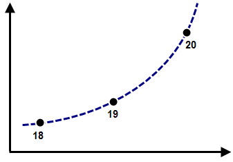
where d 0 is the initial position, V 0 is the initial velocity, A is the constant velocity, and t is the time. Note that for a constant acceleration, two points on the load curve are not sufficient; the displacement is nonlinear with time, so linear interpolation will not lead to a constant acceleration. To produce a smooth, theoretical acceleration, the time step on the load curve must be smaller than the smallest time step that occurs during the analysis. See Figure 1.
|
displacement |
| (a) The displacements at time steps 18, 19, 20 are defined in the load curve to follow the theoretical acceleration (dashed curve). If the analysis uses the same time steps, then the calculated displacement also follows the theoretical acceleration. |
|
displacement |
| (b) When the analysis reduces the time step, the displacement at the intermediate steps (steps 19 and 21) are linearly interpolated from the load curve data points (steps 18, 20, 22). Between steps 18 and 20, a linear displacement results in a constant velocity, zero acceleration. Between steps 20 and 22, a different constant velocity, zero acceleration results from interpolating the load curve. At step 20, the sudden change in velocity can result is high forces and convergence problems. |
| Figure 1: Displacement Load Curve to Simulate Acceleration |
 time
time 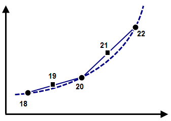 time
time Applying a Prescribed Displacement
If you have nodes, edges, surfaces, or parts selected, you can right-click in the display area and select the Add pull-out menu. Select the Prescribed Displacements command.
Determine if you want the prescribed displacement to apply a translation or rotation to the node by selecting the appropriate radio button in the Type section. Naturally, a rotation can only be applied to a node of an element that has rotational degrees of freedom, such as a beam or shell element.
Specify the magnitude of the prescribed displacement that will be applied to each selected item in the Magnitude field and the direction of the prescribed displacement in the Direction section. If you select the Scalar X, Scalar Y, or Scalar Z radio button, only the translation or rotation in that direction will be constrained; the other directions will be free to move. If you select the Vector radio button, the translation or rotation in all three directions will be constrained. For example, if you add a prescribed displacement of magnitude -1 inch and select the Scalar Y radio button, the analysis will result in a reaction force along the Y direction only. The node will be free to move along the X or Z directions. If you add a prescribed displacement of magnitude 1 inch and select the Vector radio button and define a vector of (0,-1,0), the analysis will result in reaction forces in the X, Y and Z directions. The translation in the X and Z directions will be kept at 0.
Specify the load curve that will be used to multiply the magnitude in the Load Case / Load Curve field. Press the Curve button to define a load curve in Load Curve Editor, or use the
Setup Model Setup Parameters
Analysis Parameters dialog.
Model Setup Parameters
Analysis Parameters dialog.
Tip
Since a prescribed displacement can be activated at any time through the analysis (using the birth time on the active range, see below), the model would be unstable or produce unpredictable results if the displacement at time T was to suddenly move the node from its previous position to the position implied by the prescribed displacement's magnitude multiplied by the load curve multiplier. Thus, prescribed displacements do not use the typical rule of the load at time T equals the load's magnitude times the load curve multiplier [D(T) = mag x LCM(T)]. Instead, the motion during the time step equals the prescribed displacement's assigned magnitude multiplied by the change in the load curve multiplier [ΔD(T) = mag x LCM(T)-LCM(T-1)]. So, regardless of the prescribed displacement's magnitude, these two load curves indicate that the node does not move (is held in place) for the first two seconds of the analysis:
| Load Curve 1 | ||
| Index | Time | Multiplier |
| 1 | 0 | 5 |
| 2 | 2 | 5 |
| 3 | 2.5 | 6 |
| Load Curve 2 | ||
| Index | Time | Multiplier |
| 1 | 0 | 0 |
| 2 | 2 | 0 |
| 3 | 2.5 | 2 |
Between 2 and 2.5 seconds, load curve 1's multiplier changes by a factor of 1 (= 6-5). If the prescribed displacement magnitude that is assigned to follow load curve 1 is 5 mm, then the node will move 5 mm between 2 and 2.5 seconds (= 5 mm x (6-5)).
Using load curve 2, the multiplier changes by a factor of 2 between 2 and 2.5 seconds. Thus, a prescribed displacement of magnitude 5 mm would move the node a total distance of 10 mm during this interval (= 5 mm x (2-0)).
In another example, imagine a different prescribed displacement that is activated (birth time) at 2.25 seconds. Since it is free to move during the first 2.25 seconds, imagine that the X displacement at a time of 2.25 seconds is 0.3481 inches. (This is due to other imaginary loads in the model.) Using load curve 1 with a prescribed displacement magnitude of 0.1 inch, the node will move to an X position of 0.3981 inch (= 0.3481 inch + 0.1 inch x (6-5.5), where 5.5 is the load curve multiplier interpolated at a time of 2.25 seconds).
Assign the prescribed displacement to an active range by setting the number in the Active Range field. Note that all prescribed displacements assigned to active range 1 will have the same birth and death time, the ones assigned to active range 2 will have the same birth and death time, and so on. It does not matter when the prescribed displacement is applied to the model; if multiple displacements are assigned to active range 1, they will have the same birth and death times.
Press the Data button next to the Active Range field to specify the active range (the time span) for the prescribed displacement. The Index number or row of the spreadsheet correspond to the active range number assigned to the displacement. In the Birth Time column, specify the time at which you want the prescribed displacement to start following the load curve. The magnitude and direction of the prescribed displacement will begin to be applied to the node from its current location at this time. In the Death Time column, specify the time at which the prescribed displacement will become inactive (removed from the analysis). For the prescribed displacement to become active again, specify a value in the Rebirth Index column. This will refer to another Index row. The prescribed displacements will become active again at the time specified in the Birth Time column for this index.