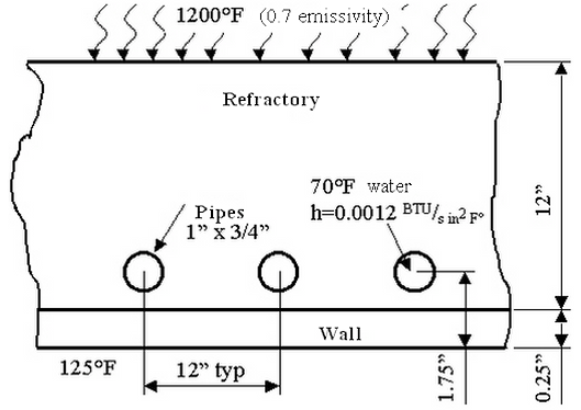
Given: A water-cooled, refractory wall in a furnace is subjected to the conditions shown in the following figure. Assume that the cold face remains at 125°F.
Find: The heat gained by the water per foot of pipe.
Problem Geometry
| Material | Wall (Part1) | Refractory (Part 2) | Pipe (Part 3) |
|---|---|---|---|
|
Conductivity (BTU/s in °F) |
6.254E-4 |
1.1E-5 |
6.254E-4 |
| Table 1: Material Properties | |||
This example only covers setting up and performing the analysis. For instructions on building the model, see Water-Cooled Wall with Radiation, Convection and Temperature Model. If you have not built the model, you can open the wcwall_input.ach file in the Models subfolder of the Autodesk Simulation installation directory.
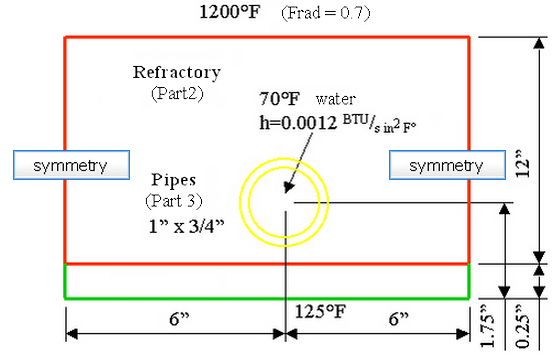
Assume that each cross section is identical. Due to symmetry, only the cross-section around a single pipe is modeled, as shown in the following figure.
- The assumed wall temperature can be fixed with nodal applied temperatures, but first estimate what stiffness is appropriate (and then confirm the results after the analysis). Generally, the stiffness is two to three orders of magnitude higher than the conductivity of the material. A stiffness of 0.625 is acceptable.
- Select the nodes at the bottom of the wall using Selection
 Shape Rectangle. Draw a rectangle that encloses the nodes at the bottom of the wall.
 - Right-click in the display area and select Add Nodal Applied Temperatures.
- In the Magnitude field, type 125 and 0.625 in the Stiffness field and click OK. The applied temperature symbol (T) appears on all the selected nodes. It keeps these nodes at 125°F.
- In the tree view, click the heading for Part 1. Hold down the Ctrl key and click the heading for Part 2. Right-click the headings and select Edit Element Type 2-D.
- With the headings still selected, right-click and select Edit Element Data. Although the thickness of the part has no affect on the temperature distribution, it does affect the surface area and the total heat flow. Type 12 in the Thickness field. Click OK.
- In the tree view, right-click the heading for Part 3 and select Edit Element Type 2-D. With the heading still selected, right-click and select Edit Element Data. Type 12 in the Thickness field. To sum the heat flow through the inside face, select the Linear Based on BC option in the Heat Flow Calculation drop-down menu. It forces the heat flow output to be based on the convection boundary conditions instead of based on the temperature distribution in the elements. Click OK.
- In the tree view, click the heading for Part 1. Holding down the <Ctrl> key, click the heading for Part 3. right-click a heading and select Edit Material. Click the Edit Properties. Type 6.254e-4 in the Thermal conductivity field. The other values are not needed for steady-state analysis. click the OK twice.
- Right-click the heading for Part 2 and select Edit Material. Click the Edit Properties. Type 1.1e-5 in the Thermal conductivity field. The other values are not needed for steady-state analysis. Click OK twice.
- Using Selection Shape Point or Rectangle and Selection Select Surfaces, click the top surface of Part 2. Right-click in the display area and select Add Surface Radiation Load. Type 1200 in the Temperature field and type 0.7 in the Function field. click the OK.
- Click the inner surface of the hole. right-click in the display area and select Add Surface Convection Load. Type 0.0012 in the Temperature Independent Convection Coefficient field and type 70 in the Temperature field click OK.
- Right-click the Analysis Type heading in the tree view and select Edit Analysis Parameters.
- Click the Options tab and type 1190 in the Default nodal temperature field. Although it is strictly not necessary in this model, we can guess that the hot face is around this temperature. By specifying an initial temperature, we will speed up the iterative process when radiation is included in the analysis. (A warning message says that the temperature value seems high. Click OK to close it).
- Because a nonlinear effect is included in the analysis (radiation), the iteration controls must be set. Click the Advanced tab and perform the following steps:
- Activate the Perform check box.
- Select the Stop when corrective norm < E1 (case 1) option in the Criteria drop-down box. It indicates that the solution has converged when the average temperature change at a node is smaller than the corrective tolerance. (Note: Other models require a difference convergence criteria.)
- Type 20 in the Maximum number of iterations field. After the analysis is completed, check that the analysis did converge within 20 iterations.
- Type 0.01 in the Corrective tolerance field. When the average temperature difference from one iteration to the next is less than this value, the solution is converged.
- Type 0.95 in the Relaxation parameter field. (Any value around 0.5 to 1 works for this model. If the model is slow to converge, try a different value.)
- Click OK to accept the input.
- Select Analysis Analysis Run Simulation to perform the analysis.
- When the analysis completes, the model is loaded in the Results environment. First we must go to the Report environment to verify that the solution has converged. Use Tools Environments Report. Click the Summary heading. Scroll near the bottom of the file and search for the text CONVERGED SOLUTION OBTAINED. It occurs on nonlinear iteration number 5. Thus, the model converged within the 20 iterations specified.
- Use Tools Environments Results to return to the Results environment.
- To read the actual values at the appropriate nodes, use Results Inquire Inquire Current Results. In particular, click the nodes across the bottom (cold face of the wall) to read the value. Since the temperatures are very close to the specified value of 125 degrees, the stiffness value used for the applied temperatures was satisfactory. Thus, with a converged solution and the stiffness value sufficiently large, the model solution is acceptable.
- To look at the total heat flowing into the water, use Results Contours Heat Flow Heat Rate Through Face.
- To see things more clearly, select View Navigate Zoom Window and draw a box around the pipe.
- To get an accurate sum, deactivate the smoothing of the results. Use Results Contours Settings Smooth Results.
- Use Selection Select Surfaces and Selection Shape Point or Rectangle and click the interior surface of the pipe.
- Select the Sum option in the Summary: drop-down box in the Inquire: Results screen. The results are approximately 8.28E-2 Btu/s. Since our model is 12 inches thick, it is the heat rate per foot of pipe.
An archive of this model (wcwall.ach) with results is located in the Models subfolder of the Autodesk Simulation installation directory. To retrieve the file, use  Archives Retrieve in the FEA Editor environment and then select the file.