After the simulations have finished, we can begin to examine results. First we will start with the zero degree model.
- Inside Abaqus, click and select bar_zero_output.odb. This will open the output database in the Visualization module.
- Click to display the contour plot.
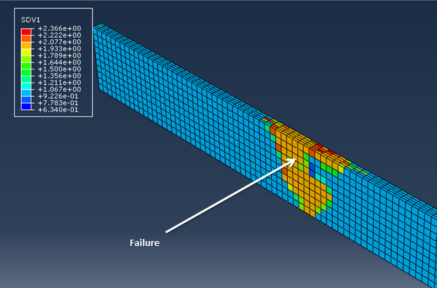
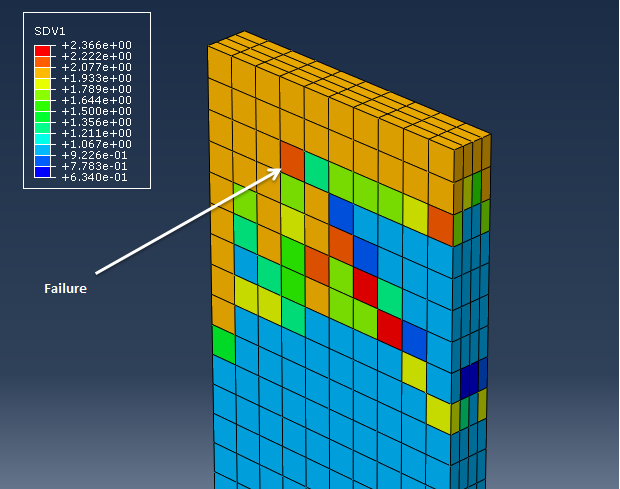
- Now select SDV1 from the list of output variables (). SDV1 represents the rupture state of the material, where 1 = Not Ruptured and 2 = Ruptured.
- Step through the load history to see the progression of failure in the bar.
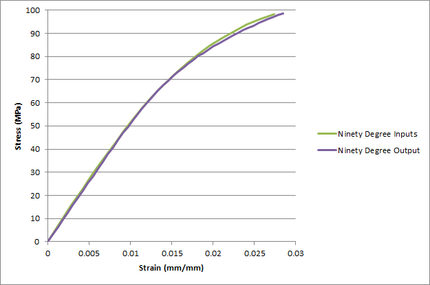
Now we can create a stress-strain plot to compare to the idealized curve produced with Advanced Material Exchange.
- Select . In the dialog box that appears, select the ODB field output option and click Continue.
- In the dialog box that appears, select Unique Nodal for the Position and check the RF2 and U2 check boxes. On the Elements/Nodes tab, choose Node Sets and select the LOAD_NODE.
- Click Save, click OK, and click Dismiss.
- Now we can copy the data to a spreadsheet, calculate the stress and strain based on the dimensions of the coupon, and plot the results.

We see a good representation of the nonlinear stress-strain data in the output results. If we remember the zero degree curve fit produced by Advanced Material Exchange, the output results align very well. It is also important to keep in mind that the fiber orientations in the coupon were not aligned perfectly at zero degrees. This will also contribute to the difference seen in the input and output curves. The ability to capture the nonlinear behavior of the fiber filled material is very important to the accuracy of the structural analysis.
Now we can repeat the steps above for the bar_ninety_output.odb file. The plots of SDV1 and the stress-strain curve are shown below. Once again, good agreement is found between the input stress-strain data and the results produced from the simulation.