- After the solution has completed, click .
- First, we will focus on the composite damage. To view a contour plot of SVAR1, type PLESOL, SVAR, 1 into the command prompt. Click if necessary.
SVAR1 represents the damage state of the material. For a unidirectional composite material, SVAR1 can take the values of 1.0 (no failure), 2.0 (matrix failure), and 3.0 (fiber failure).
- Change the plot contour settings to correspond to the three composite damage states. Click and enter V1 = 1, V2 = 2, V3 = 3. Click OK. This will allow for easy determination of constituent failure. Blue elements represent an undamaged composite, green elements represent matrix failure, and red elements represent fiber failure.
- Step through the load history and note the progression of SVAR1 as more load is applied ( or use the SET command).
- The first failure to the fiber and matrix occurs in the top group of 0 degree plies at a step time of 0.33.
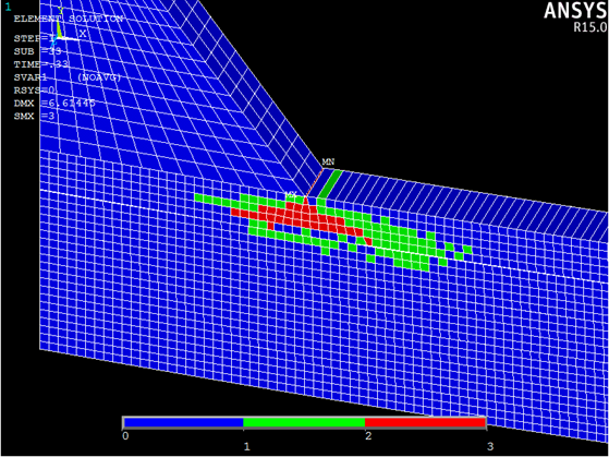
- The first failure to the fiber and matrix occurs in the top group of 0 degree plies at a step time of 0.33.
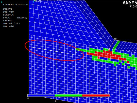
- Now we can examine the cohesive layers.
- At a step time of 0.40, we clearly see the first delamination between the 0 and 90 degree ply groups on the top of the beam.
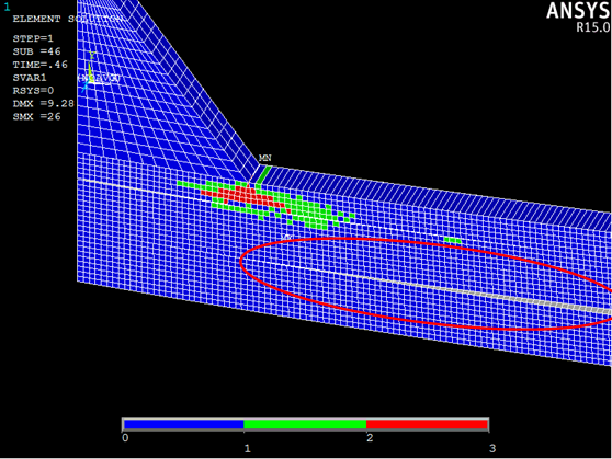
- We see the second large delamination occur at a step time of 0.46.
- At a step time of 0.40, we clearly see the first delamination between the 0 and 90 degree ply groups on the top of the beam.
There are several solution variables useful for viewing results of cohesive materials. In particular, SVAR2, the failure index used for determining damage initiation, and SVAR6, the damage variable which indicates when complete stiffness loss occurs. To examine the cohesive solution variables, it is best to display only the cohesive elements from the viewport (). For a complete list of the solution variables used in the analysis, refer to the .mct file.