View and Interpret Results

View the results of the analysis in the steps that follow.

Simulation Composite Analysis generates several state variable outputs. In this step, a key variable (SDV1) is viewed and discussed. SDV1 is the state variable that tracks fiber and matrix failure within an element.

1. After the job has completed, click File > Open from the main toolbar and open ASCA_Tutorial_1_Abaqus_xs.odb. This will open the output database file and switch to the Visualization module. The undeformed plate appears in the viewport.
2. State variable SDV1 is used to identify the discrete damage state of the composite material. To plot this variable, select Result > Field Output from the main toolbar. The Field Output dialog box appears.
3. Select SDV1 from the list of Output Variables. Click OK.
4. The elements appear to be heavily distorted because the deformation scale factor is set too high. Adjust the Deformation Scale Factor by selecting Options > Common and entering a value of 1 in the Deformation Scale Factor field. Click OK.
5. The default Contour Type is Banded, but the Quilt type is more useful for viewing SDV1 output. To switch from Banded to Quilt, select Options > Contour from the main toolbar, and select Quilt as the Contour Type. Click OK. The plot should be similar to that shown below. Minor differences are usually the result of mesh variations.

The following table lists three possible values for SDV1 and the corresponding failure states. It can be helpful to decrease the number of Contour Intervals to 3 and specify user-defined limits so the element colors remain consistent. For example, if there are 12 intervals and only matrix failure, Abaqus will automatically adjust the limits to range from 1 to 2 and red elements will correspond to matrix failure but when fiber failure occurs, the range will be adjusted to 1-3 so that red elements correspond to fiber failure instead of matrix failure. By setting the number of Contour Intervals to 3 and specifying appropriate user-defined limits, the range of values of SDV1 will be always be 1 to 3.

Value of SDV1	Failure State
1	No Failure
2	Matrix Failure
3	Fiber and Matrix Failure



Note: the default ply for the contour plot shown above is Ply-1. To view failure in all of the plies, envelope plots can be used. Envelope plots display the maximum or minimum integration point value across all section points in each element.
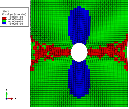
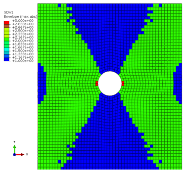
6. Select Result > Section Points from the main toolbar to create an envelope plot. Select the Envelope option from the Categories box and click Apply. The plot should be similar to that shown below.

   

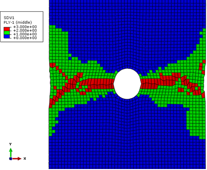
7. To view the failure state of a single ply, click Plies from the Section Points dialog box. View the failure in each ply. Note that plies with the same orientation have identical failure states since the laminate is symmetric. For example, Ply-2 and Ply-23 have the same failure states.

   Viewing the progression of failure is often useful for visualizing the way a structure fails.

8. Switch back to the envelope plot.
9. Select Result > Step/Frame from the main toolbar. A list of each increment in the step appears.
   • As an alternative, the step controls on the toolbar can be used.
10. Starting at Step Time = 0.000, progress through the step while watching the viewport to determine when failure initiates and how failure propagates.
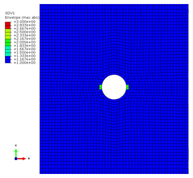
    • First matrix failure should occur at Step Time = 0.25 (First image below).
    • First fiber failure should occur at Step Time = 0.65 (Second image below).

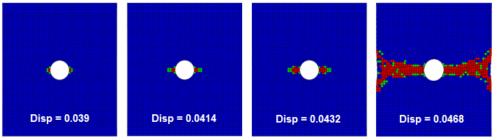
Next, consider the progression of failure in ply-2, which is one of the main load carrying (0°) plies. The plot below shows failure in ply-2 at several displacements. As expected, failure initiates at the corners of the notch and progresses laterally towards the edge of the plate until ultimate failure.