View contour plots of the MCT state variables.
MCT state variables are element output variables stored at every integration point within each element. Consequently, the same familiar methods used to view stress and strain fields at each time increment can be used to view MCT state variables. However, to view MCT state variables in Abaqus/Viewer, the Abaqus input file must first request that they be written to the Abaqus output database file (see Request MCT State Variable Output for Composite Materials and Request MCT State Variable Output of the MCT State Variables). For a complete description of each of the MCT state variables, refer to Appendix C.
Contour plots are usually the most appropriate means of examining the distribution of the MCT state variables. To generate a contour plot within Abaqus/Viewer, click the contour icon  or select from the main toolbar. The default variable Abaqus/Viewer plots is the von Mises stress. To view MCT state variables computed by Simulation Composite Analysis, open the Field Output dialog box by selecting from the main toolbar. MCT state variables (SDV1, SDV2, SDV3, …, etc.) are listed within the Field Output dialog box along with more familiar variables such as stress (S) and strain (E). The number of SDVs available in the Field Output dialog box depends entirely on the number of SDVs that were requested by the Abaqus input file via the *DEPVAR keyword statement.
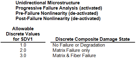
The fundamental MCT state variable is SDV1 which indicates the discrete damage state of the composite material. SDV1 is a real variable that can assume a finite number of discrete values between 1.0 ≤ SDV1 < 4.0. The specific set of discrete values that can be assumed by SDV1 depends upon the type of composite material (unidirectional or woven) and the specific set of material nonlinearity features used by Simulation Composite Analysis during the finite element solution (see Appendix C). An MCT file (*.mct) is generated when an analysis enhanced with Simulation Composite Analysis is submitted and contains the specific set of values that can be assumed by SDV1 for each material in the model.
It should be noted that contour plots of fully-integrated elements can show values of SDV1 that are less than 1 and greater than 4. This is entirely due to the scheme Abaqus uses to compute contour values. For element-based values, such as SDV1, the computations vary depending on several criteria. In general, the extrapolation of integration point values to the nodal locations is the reason SDV1 can be less than 1 and greater than 4 for fully-integrated elements. To view the exact values for SDV1 at each integration point within a specific element, use the Probe Values tool in the Abaqus Query toolset.
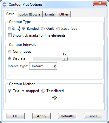
Because SDV1 is a discrete real variable taking values 1.0 ≤ SDV1 < 4.0, it is important to change the settings of Abaqus/Viewer so that a unique color contour is associated with each discrete integer value of SDV1. In the case where SDV1 can assume values of 1.0, 2.0, or 3.0, set the number of color contours to 3. The number of contour intervals used in a contour plot can be specified from the Contour Plot Options dialog box, which is accessed by clicking from the main toolbar. The Contour Plot Options dialog box is shown below. Under the heading 'Contour Intervals', choose 'Discrete' and use the slider bar to select the number of discrete color contours to match the number of integer values SDV1 can assume.
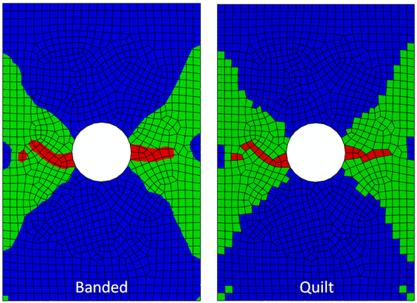
The image below shows two different contour plots of the integer variable SDV1 for an axially loaded composite plate with a central hole. The use of three discrete colors makes it easy to identify the regions where each discrete composite damage state occurs. The blue elements (SDV1=1) are completely undamaged; the green elements (SDV1=2) have failed matrix constituents and undamaged fibers; the red elements (SDV1=3) have failed matrix constituents and failed fiber constituents. Note that the quilt contour plot shows the average value of SDV1 for each individual element, while the banded contour plot simply uses the values of SDV1 at the individual integration points to establish the color contours independent of the element boundaries.
The remaining MCT state variables (SDV2, SDV3, SDV4, …,SDV90) are continuous real variables. Therefore, in generating contour plots of these variables, it is not critical to manage the number of color contours. Furthermore, the standard practices used in viewing stress and strain distributions are also appropriate for viewing SDV2, SDV3, SDV4, …, etc..
Selection of Section Points
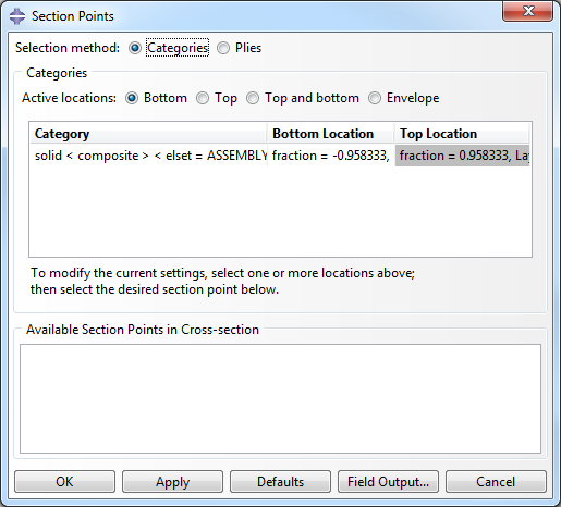
When viewing finite element solution results for laminated composite structures, you must be aware of the numbering of section points through the thickness of multilayer elements. A contour plot will only use the values of the variable stored at a particular section point. Therefore, to view a contour plot for a specific material layer, you must choose a section point that lies within that material layer. To choose a specific section point, access the Section Points dialog box by selecting from the main toolbar. The Section Points dialog box is shown below. The default section point plotted by Abaqus/Viewer is the bottom section point (i.e., the section point at the bottom of the element). To view results for a particular material ply, check the Plies option and select the appropriate ply. Select the Envelope option to view results for all section points in the same plot. Envelope plots show the maximum absolute, maximum, or minimum value of the selected variable across all of the plies in a layup.
As an example of the recommendations above, consider the image below. This shows envelope quilted contour plots of SDV1=1,2,3 at several points in time during a progressive failure analysis of a composite plate with a central hole. The plate has eight material plies and is loaded in tension. Since these contour plots are envelope plots, the color at any location represents the highest value of SDV1 achieved at any of the section points distributed through the thickness of the 8-ply laminate. In these plots, blue elements have no failure at any of the section points distributed through the laminate thickness. The green elements have at least one section point where matrix failure has occurred, while the red elements have at least one section point where both matrix and fiber failure occurred.
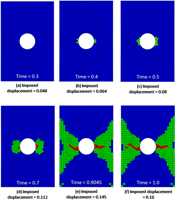
Several important observations can be made regarding the sequence of envelope quilted contour plots shown above:
- At time = 0.3, every element is blue, meaning no points in the composite plate have experienced any type of failure.
- At time = 0.4 there are some green elements at the edges of the hole. Within these green elements, at least one material ply has experienced a matrix constituent failure. However, the plot does not specify which of the material plies have experienced a matrix constituent failure.
- Comparing the plots at times 0.4 and 0.5 indicates the progression of matrix constituent failure as the load increases.
- At time = 0.7, the matrix failure has spread further, and there are three elements with fiber failure, as indicated by the red elements. Again, the red elements indicate that at least one of the 8 material plies has experienced a fiber constituent failure.
- At time = 0.9045, there is significant matrix failure, and the fiber failure has spread out towards the plate edges.
- At time = 1.0, there is additional matrix and fiber failure.