View and Interpret Results

Examine the results of the analysis.

Simulation Composite Analysis generates several state variable outputs that are stored in the output database file. In this step, these variables are viewed and discussed.

1. After the job has completed, click File > Open from the main toolbar and open ASCA_Tutorial_3_xs.odb. This will open the output database file and switch to the Visualization module. The undeformed plate appears in the viewport.
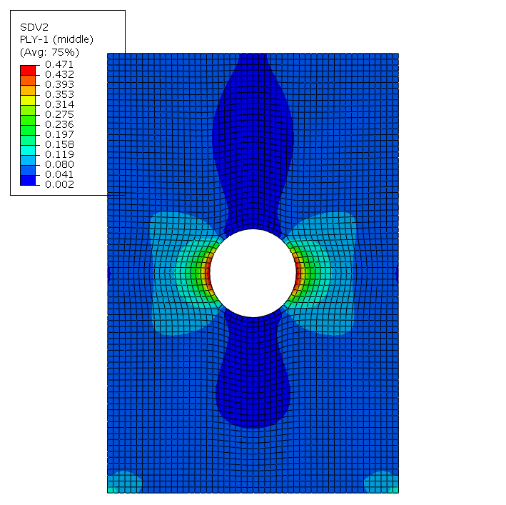
2. State variable SDV2 represents the matrix failure index. This variable indicates how close the matrix is to failure, which occurs when SDV2 is greater than or equal 1. To plot this variable, select Result > Field Output from the main toolbar. The Field Output dialog box appears. Select SDV2 from the list of Output Variables. Click OK.
3. Choose Contour from the Select Plot State dialog box that appears. Click OK.
4. Adjust the Deformation Scale Factor by selecting Options > Common from the main toolbar and entering a value of 1 in the Deformation Scale Factor field in the Common Plot Options dialog box. Click OK. The plot should be similar to the plot shown below.

Note: The default ply for the contour plot shown above is Ply-1 and the maximum SDV2 value is 0.492. This means that in Ply-1, the matrix failure index is less than 1 and no failure has been detected.

To view the maximum matrix failure index in all of the plies, envelope plots can be used. Envelope plots display the maximum or minimum integration point value across all of the section points in each element.

1. To create an envelope plot, select Result > Section Points from the main toolbar. Select the Envelope option from the Categories box and click Apply. The plot should be similar to that shown below.

   

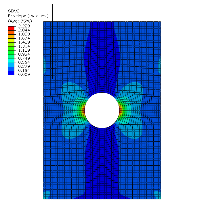
   The maximum matrix failure index is 2.226, which indicates that matrix failure is predicted to occur in one or more of the plies.

2. The step in which matrix failure first occurs can be determined by viewing results from intermediate load steps. Select Result > Step/Frame from the main toolbar. A list of each increment in the step appears. As an alternative, use the step controls on the toolbar.
3. Starting at Step Time = 0.000, progress through the steps while watching the viewport to determine when matrix failure is detected (when the maximum SDV2 value is 1 or greater). Matrix failure occurs between step time 0.65 and 0.7.
4. To determine which plies have matrix failure, click Plies from the Section Points dialog box and view the failure distribution in each ply. Note that plies with the same orientation have identical failure index distributions since the laminate is symmetric. For example, Ply-2 and Ply-7 have the same failure index distribution.

   All plies except plies 1 and 8 have matrix failure. Matrix failure is not predicted in plies 1 and 8 since these plies have their fibers oriented in the loading direction. The stiff fibers restrict the strains in plies 1 and 8 from reaching critical levels. The increment that first caused matrix failure can be determined by viewing results from intermediate load steps.

5. Switch back to the envelope plot and plot the last frame (step time = 1.00).
6. From the main toolbar, select Result > Field Output and plot SDV3. SDV3 represents the fiber failure index and is an indication of how close the fiber is to failure. Fiber failure occurs when the value of SDV3 is greater than or equal to 1. The plot should be similar to that shown below.

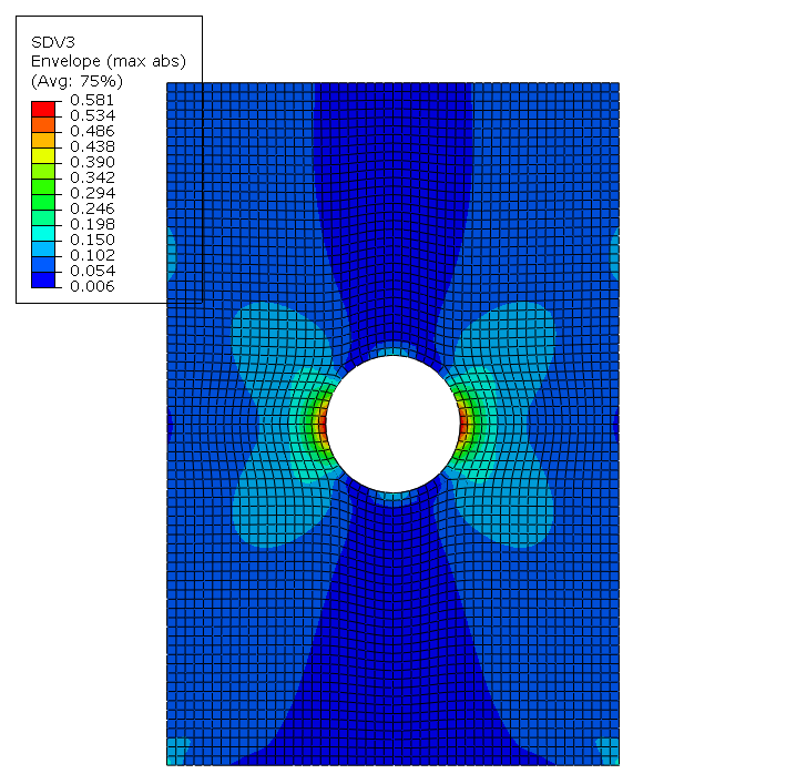
Since the maximum value of SDV3 in all plies is less than 1, fiber failure is not predicted.